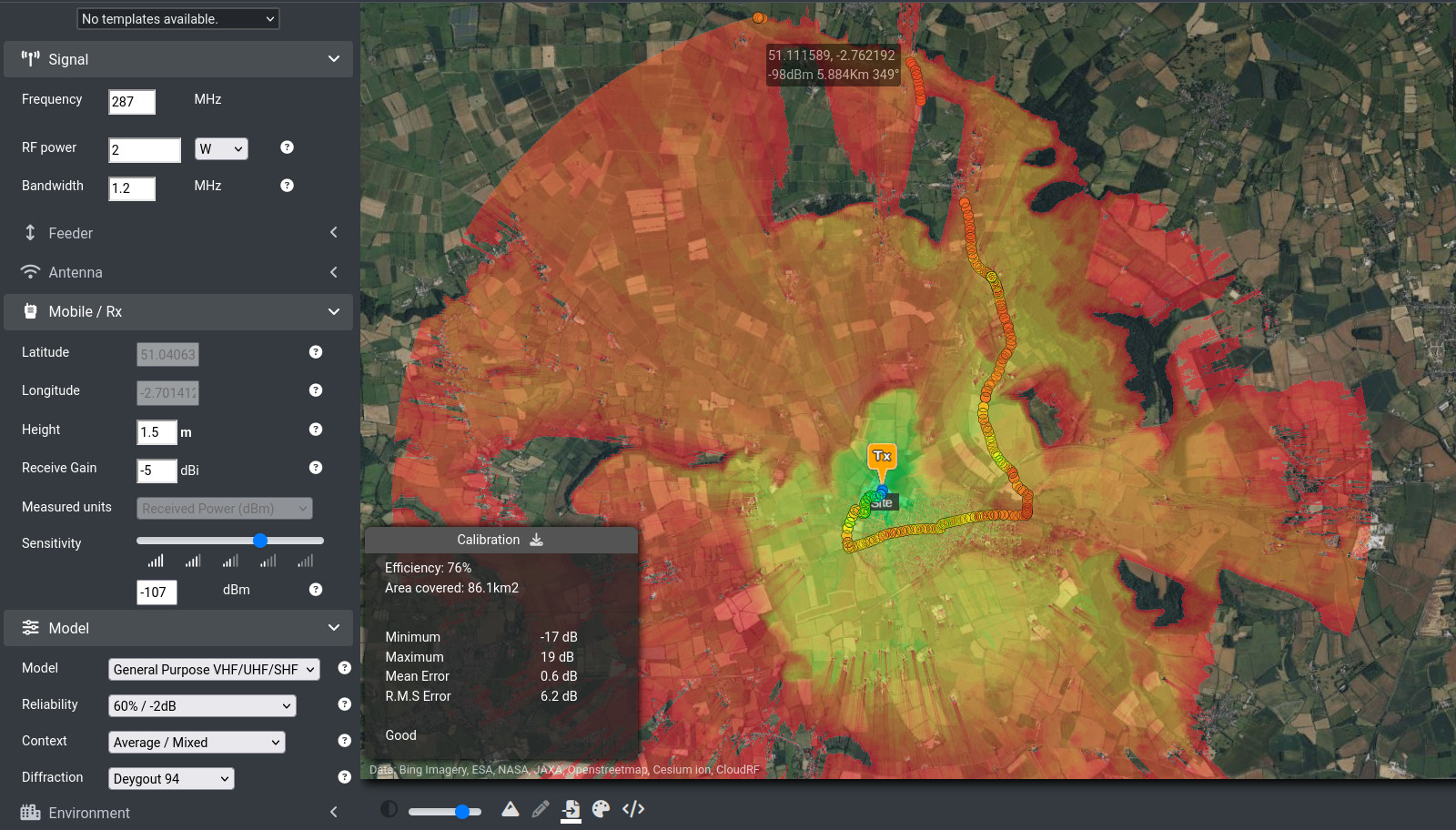
Simulating indoor radio coverage for first responders has been made simpler thanks to a new capability called Phase Tracing.
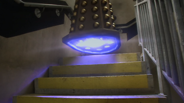
The novel design was influenced by the 2017 Grenfell Tower inferno, where radio communication in concrete stairwells was highlighted as a major problem. The Grenfell inquiry highlighted radio and training issues in the report, which had a section dedicated to communications.
During the inquiry, expert witnesses were unable to demonstrate how far a signal would travel within the tower, even with the availability of indoor planning tools. Estimated distances offered to the inquiry were based upon empirical measurements from elsewhere and were at odds with witness statements from firefighters who reported losing communication after only four floors and communicating with paper notes.
The intensive computation required to perform a true 3D simulation with reflections has been made practical through developments in graphics processing. As a result, accurate radio coverage in stairs, tunnels and elevator shafts can be simulated, at the network edge, by an operator with minimal training.
In contrast to legacy indoor planning tools, which use floor plans and images; Phase Tracing is designed for critical communications and industrial markets in challenging and dynamic 3D environments, represented by digital models.
Models not floor plans
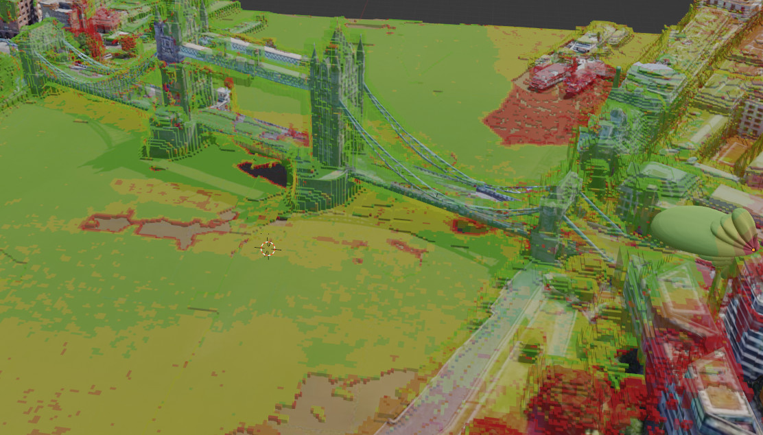
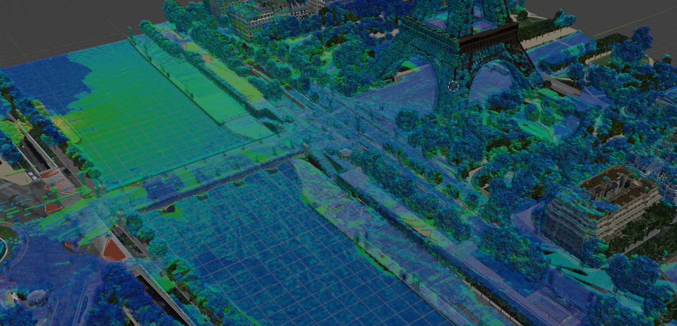
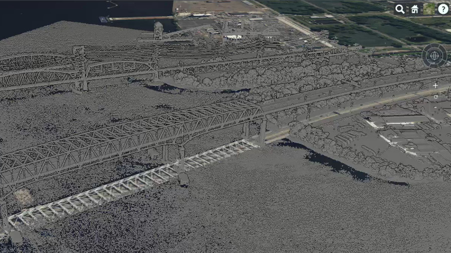
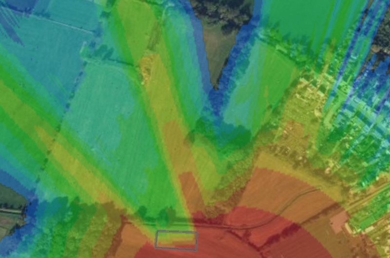
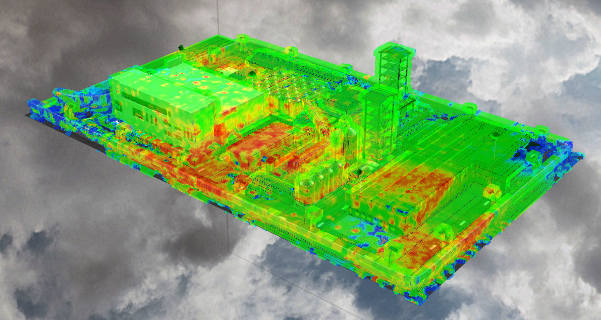
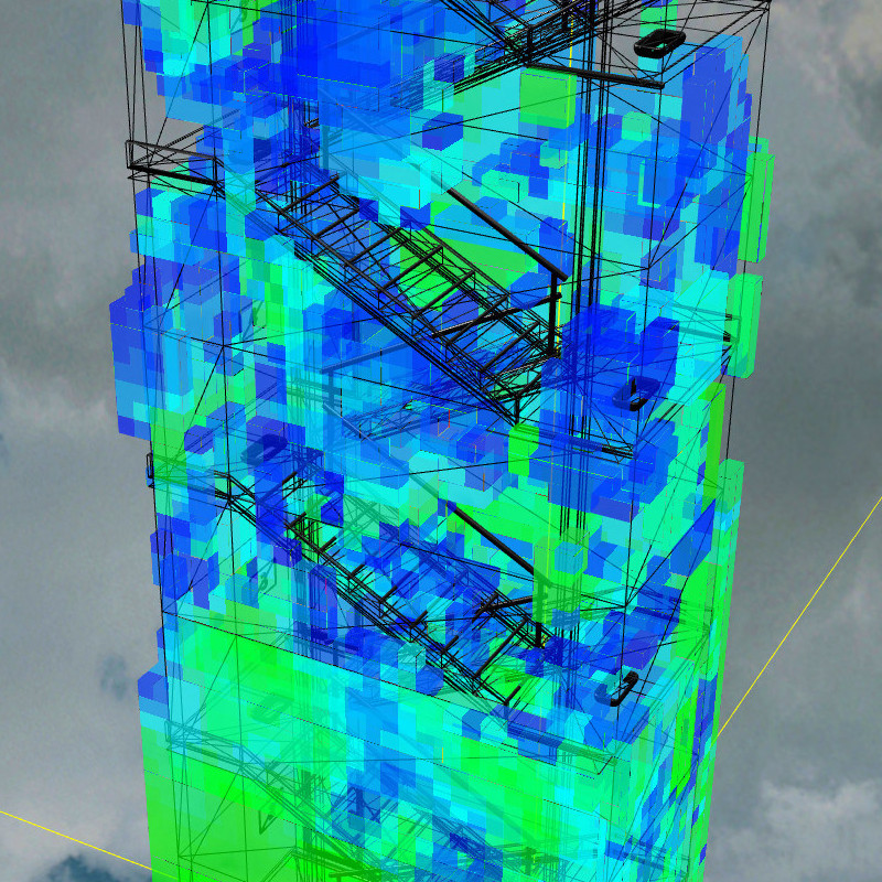
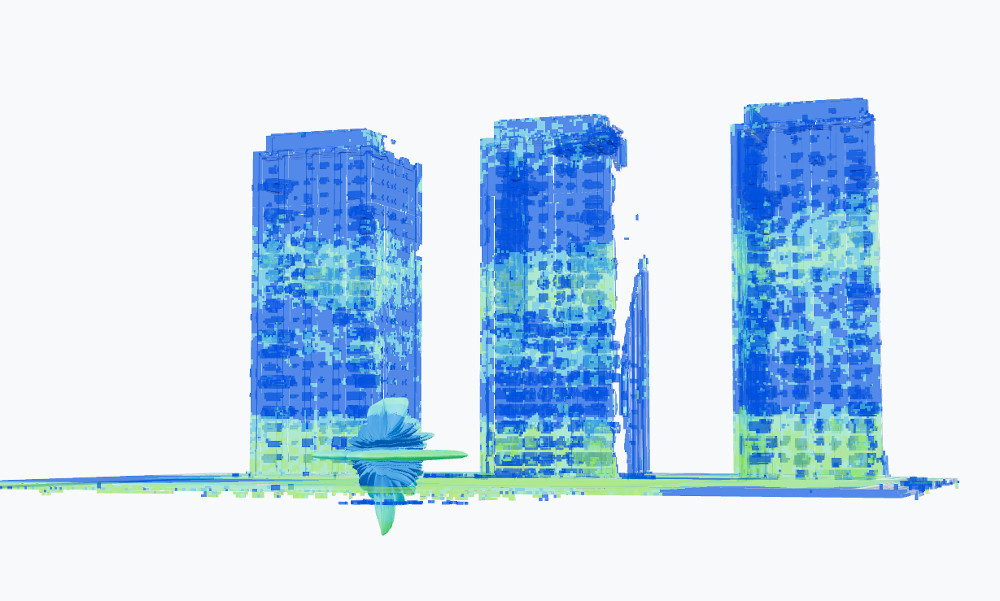
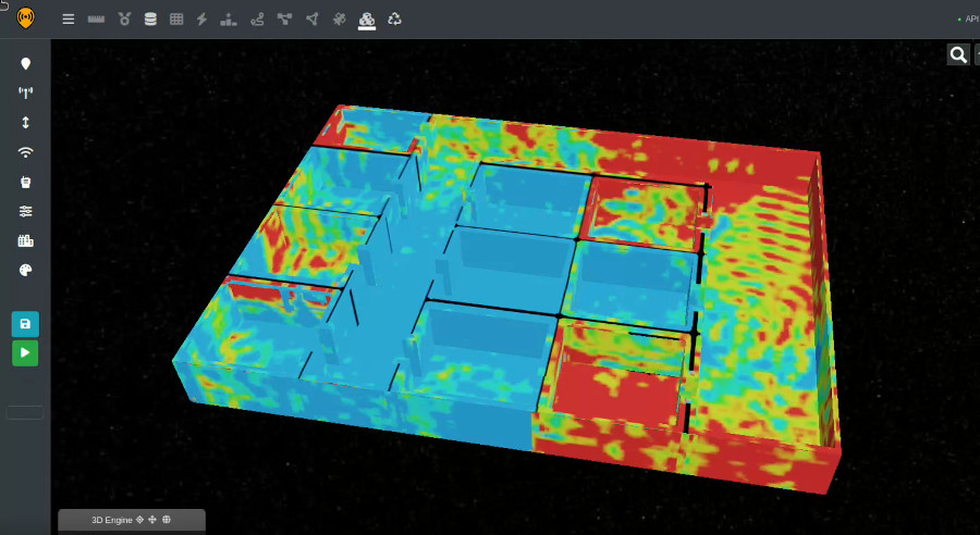
Phase Tracing represents a leap forward for radio simulation from overlaying images upon a 2D map or floor plan, suitable for an estate agent, to using a digital twin 3D model which considers all floors, and the obstructions in between from stairs, to air ducts and pylons. Simulating reflections is critical for indoor modelling which is a pillar of the design.
There also exists a huge gap in the market between indoor simulation packages and the skill required to use them effectively, and first responders who are left guessing where they will lose communications on a stairwell. This gap has been closed by developments in computation, namely GPU processors, and web technologies which mean this powerful API can be used from a low power touchscreen device.
A little movement…
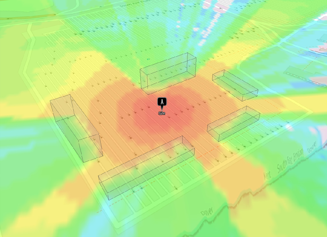
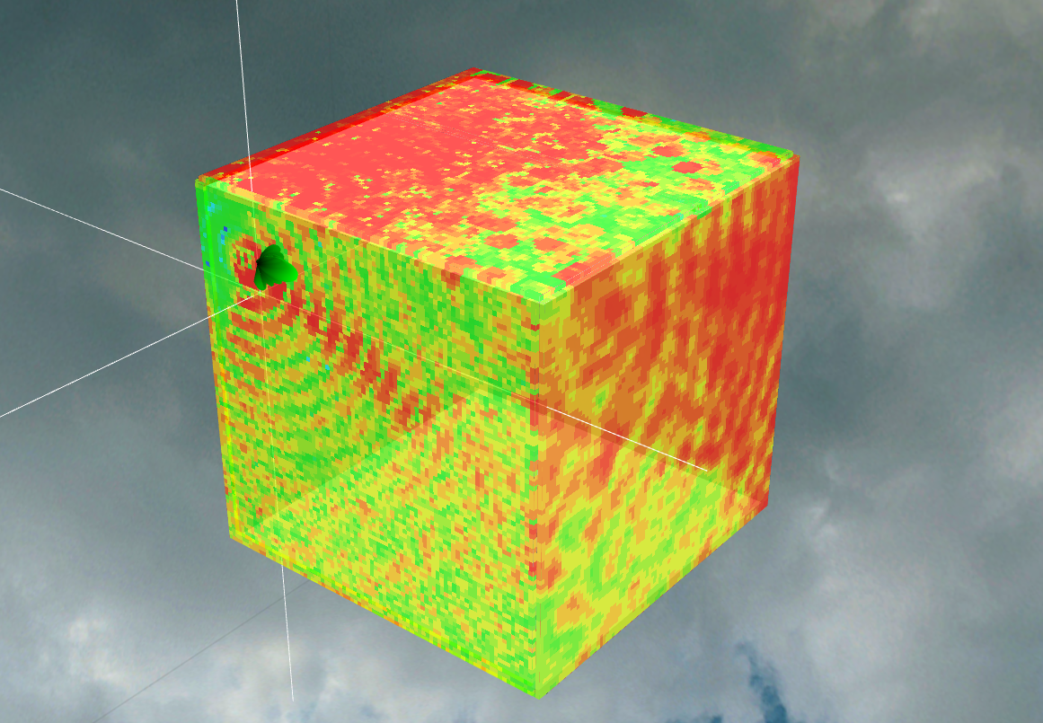
For RF theory students who are taught the impact of multi-path; they now have a tool to visualise and explore this important concept; so they can see why “a little movement may cure a dead spot”. Better still, they can identify constructive “good” multipath they didn’t know about.
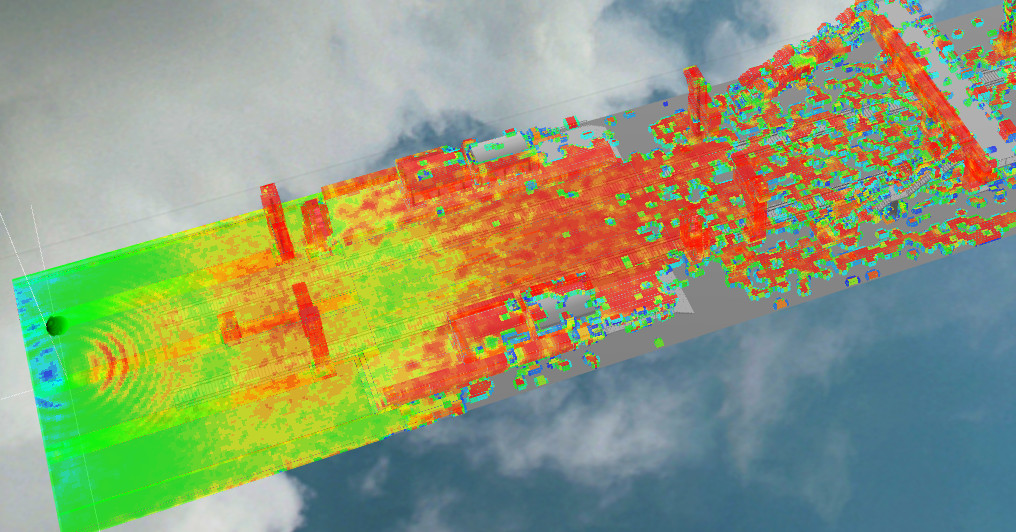
The GPU accelerated engine reads and writes to open standard glTF models and uses ray tracing techniques from computer games to bounce photons around the model. With the addition of phase, multi-path artefacts such as signal “dead spots”, where out of phase signals on the same wavelength cancel each out, can be modelled.
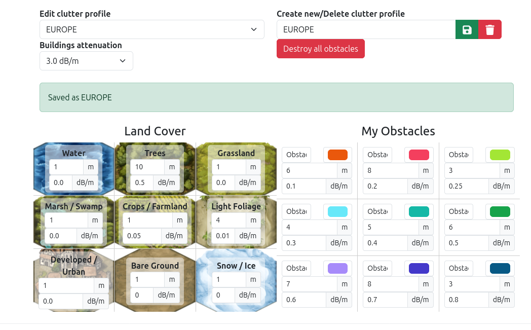
The number of reflections, material attenuation and scattering properties can be configured. This is essential for modern buildings which are built with materials which disrupt radio communication.
Applications
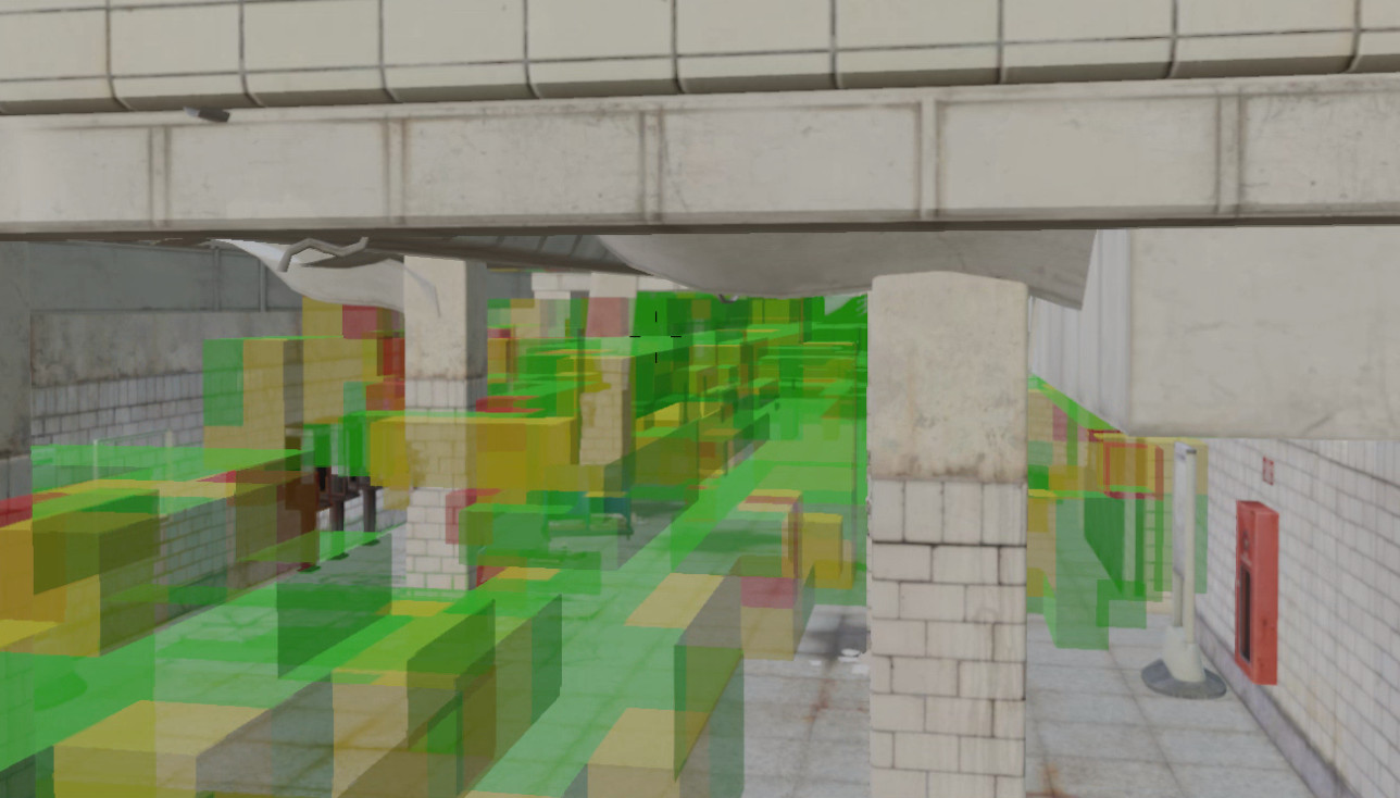
Phase Tracing has a distinct advantage over 2D modelling for the following 3D obstacles in most wireless industries.
- Stairs
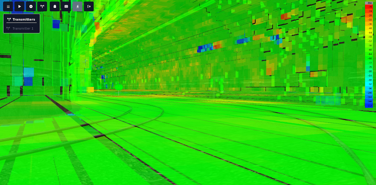
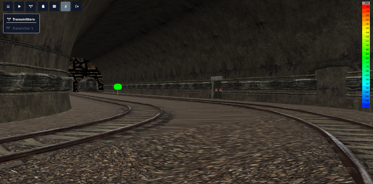
- Tunnels
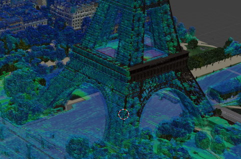
- Bridges
- Towers
- Pylons

Design
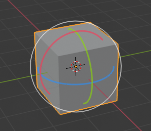
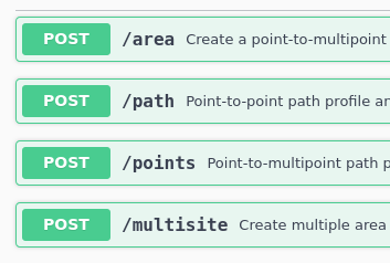
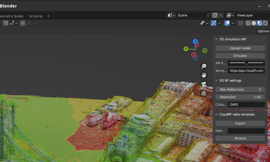
The Phase Tracing capability is built upon our 3D API which we launched last year with a blender plugin. The API can be called directly to integrate the output into other model based systems, or even viewed in a standalone HTML5 viewer.
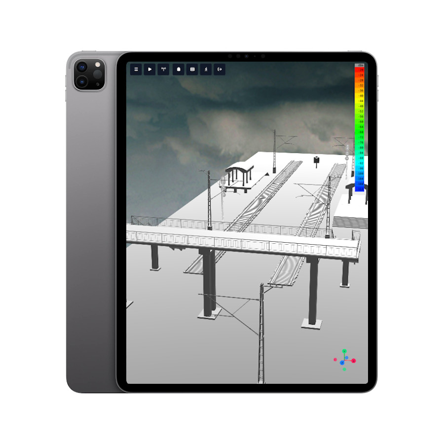
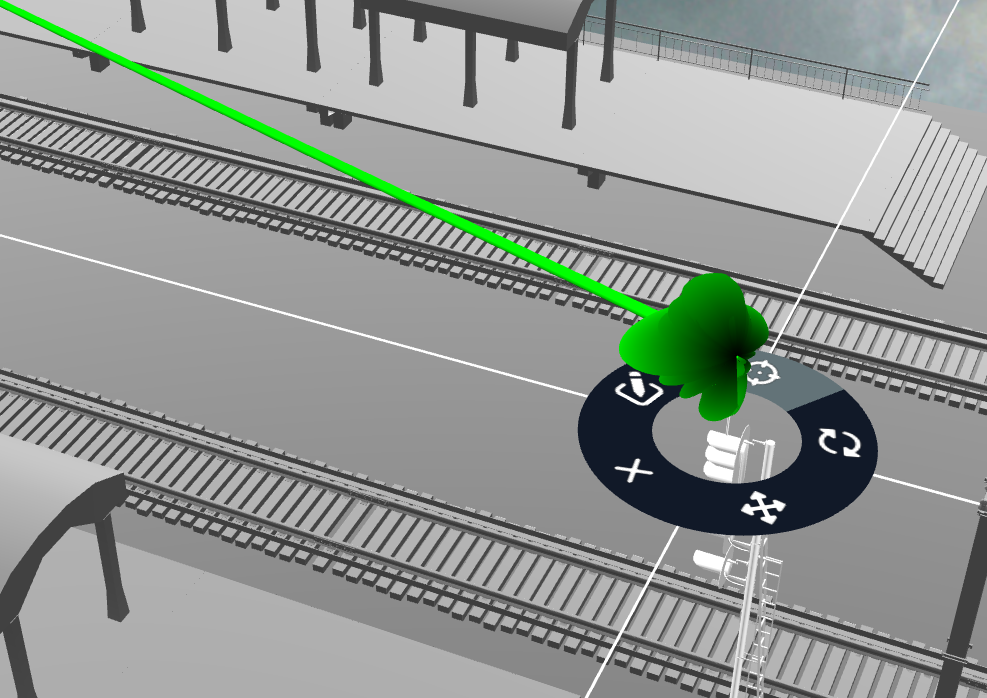
The interface and API is radically different to our map based Globe. For starters there are no Geographic coordinates, positions are in Cartesian XYZ co-ordinates relative to position 0,0,0. This is so you can work with models which might not have a geo reference or in the case of design, might not even exist yet.
Photons and Phase
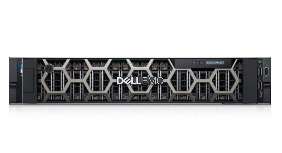
The 3D engine is a CUDA accelerated pipeline, like our 2D GPU engine, which processes jobs asynchronously to service multiple users. It creates a voxel model from a glTF file which it then radiates photons around. A photon will reflect from obstacles until it runs out of energy or reaches a reflection limit. Unlike Ray Tracing, a legacy technique for indoor modelling, these photons maintain their phase so multi-path can be simulated in all directions.
Each reflection costs several decibels of power typically so there is a practical limit, depending on the material, after which it will be too weak to be useful and the photon should be killed. The engine can model up to 30 reflections per photon which do not impact performance so much as the number of photons, currently set to 2e6. The required number of photons depends upon the model: If you have a small office and need to decide where best to put a Wi-Fi Access Point you don’t need many.
If however, you need to model reflections up a stairwell, along a corridor and into a flat you need millions. This isn’t fast, or pretty, but such is the nature of critical communications. We’ve fixed the photon limit on CloudRF to deliver a calculation in under 30 seconds for a large model. A small model will be quicker.
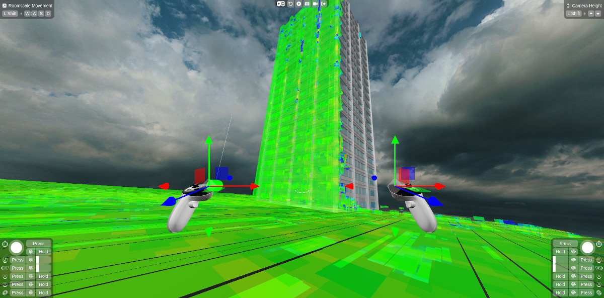
VR/AR support
The cross platform interface uses three.js and the WebXR library which supports Virtual Reality and Extended Reality devices. We have a XR branch we’re playing with on a Meta Quest but are having a headache issue as it is so immersive you get vertigo exploring tall models. Once this is sorted, likely by AR, we’ll merge it. Last year the 3D output was integrated into a third party Hologram interface.
Demo Gallery
We have an interactive demo gallery of 3D models you can explore on our Github pages. To use these demos you will need a WebGL capable web browser like Chrome. You can use your mouse to zoom in and explore the models or download them as GLB to view on your phone using an app like glTF viewer. iPhones support these GLB models natively.
Roadmap
The API and version 1.0 of the interface have been published. The API can be used by Silver and Gold customers and the interface is restricted to Gold only presently whilst we build more infrastructure to support this.
June 2024 – 3D API
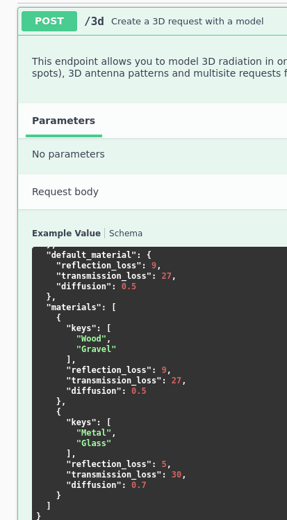
- Upload glTF model
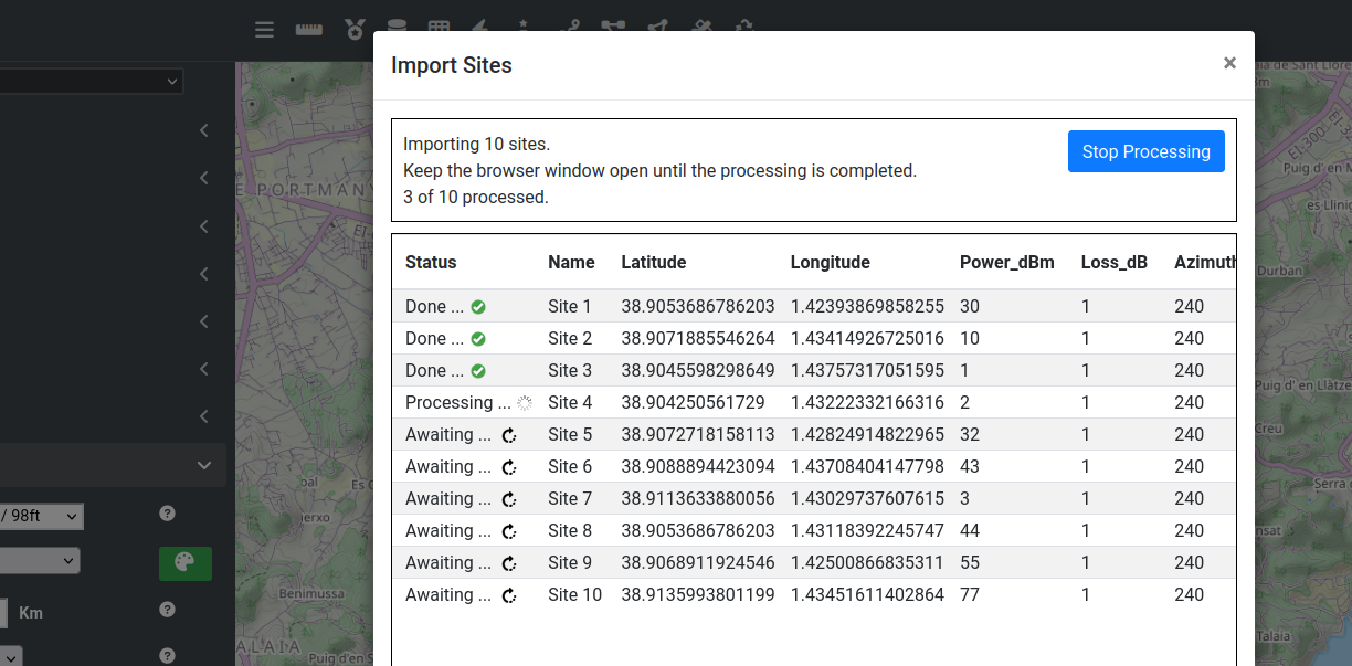
- Perform multi-site simulation using transmitter parameters
- Configurable material attenuation
- Configurable reflections and attenuation
- Blender plugin
- 1e6 photons
- Mega voxel limits
Jan 2025: Phase Tracing 1.0
- Cross platform web interface
- GLB Model management (Add, Remove)
- Local model caching
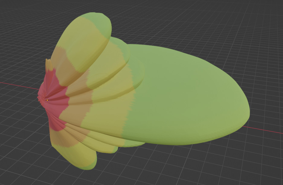
- 3D antenna models built from user’s antennas
- Click to aim
- Configurable reflections, resolution and default material density
- 2e6 photons
- Save/Load settings as JSON
TBC: Phase Tracing 1.1
- Official VR/XR support
- GLB download
- Material manager for construction materials
- Biasing for speed boost
- Configurable photon limits – linked to plan
Sample GLB models
Upload these glTF binary models into the interface or another tool such as this handy free viewer.
You can validate your models with another free tool here.
[3d_viewer id=”46074″]