Summary
We conducted a field test in the mountains with SOOTHSAYER focused on automation and endurance. The test generated quality data and revealed altitude issues with our plugin we have since fixed.
We conducted a field test in the mountains with SOOTHSAYER focused on automation and endurance. The test generated quality data and revealed altitude issues with our plugin we have since fixed.
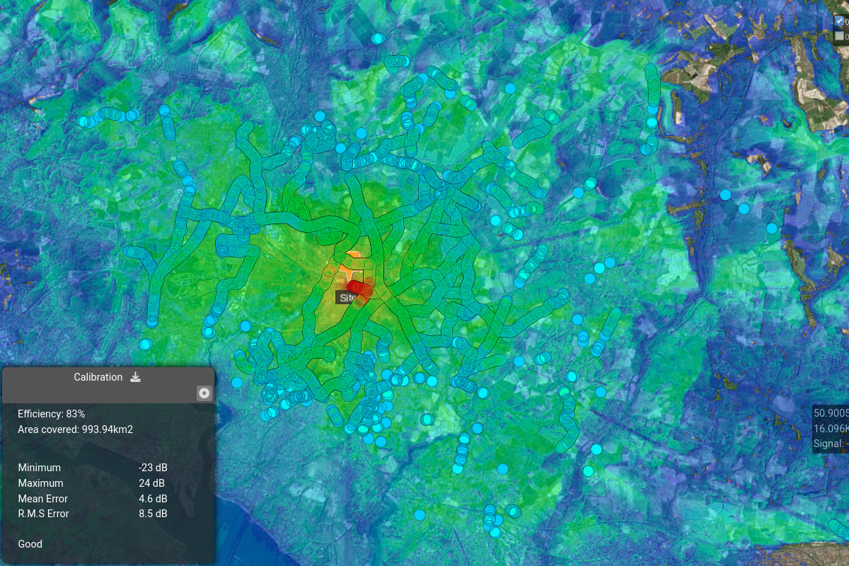
During the test we created 925 multi-site coverage heat maps and 4625 links to maintain a live map of the network. We previously established model accuracy on previous field tests so the focus here was on endurance.
Live network mapping is radio planning without user interaction where radio locations and coverage are updated dynamically via an API. It requires fast and economical edge compute like our SOOTHSAYER API to be effective and is not possible with legacy desktop tools.
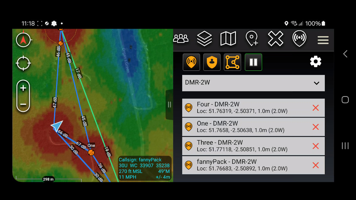
This offline edge capability is implemented in our ATAK plugin via the Co-Opt feature. This new feature updates network coverage automatically using live map data to provide a current view of communications problems and opportunities, akin to a moving weather layer. It is useful for deploying radio networks into challenging terrain.
Test objectives
- Collect performance data
- Prove software stability
- Test altitude logic
Test setup
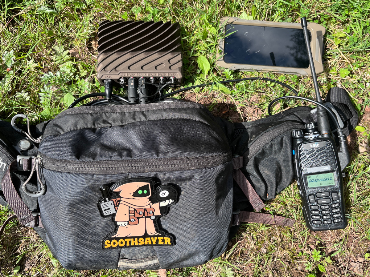
Hardware
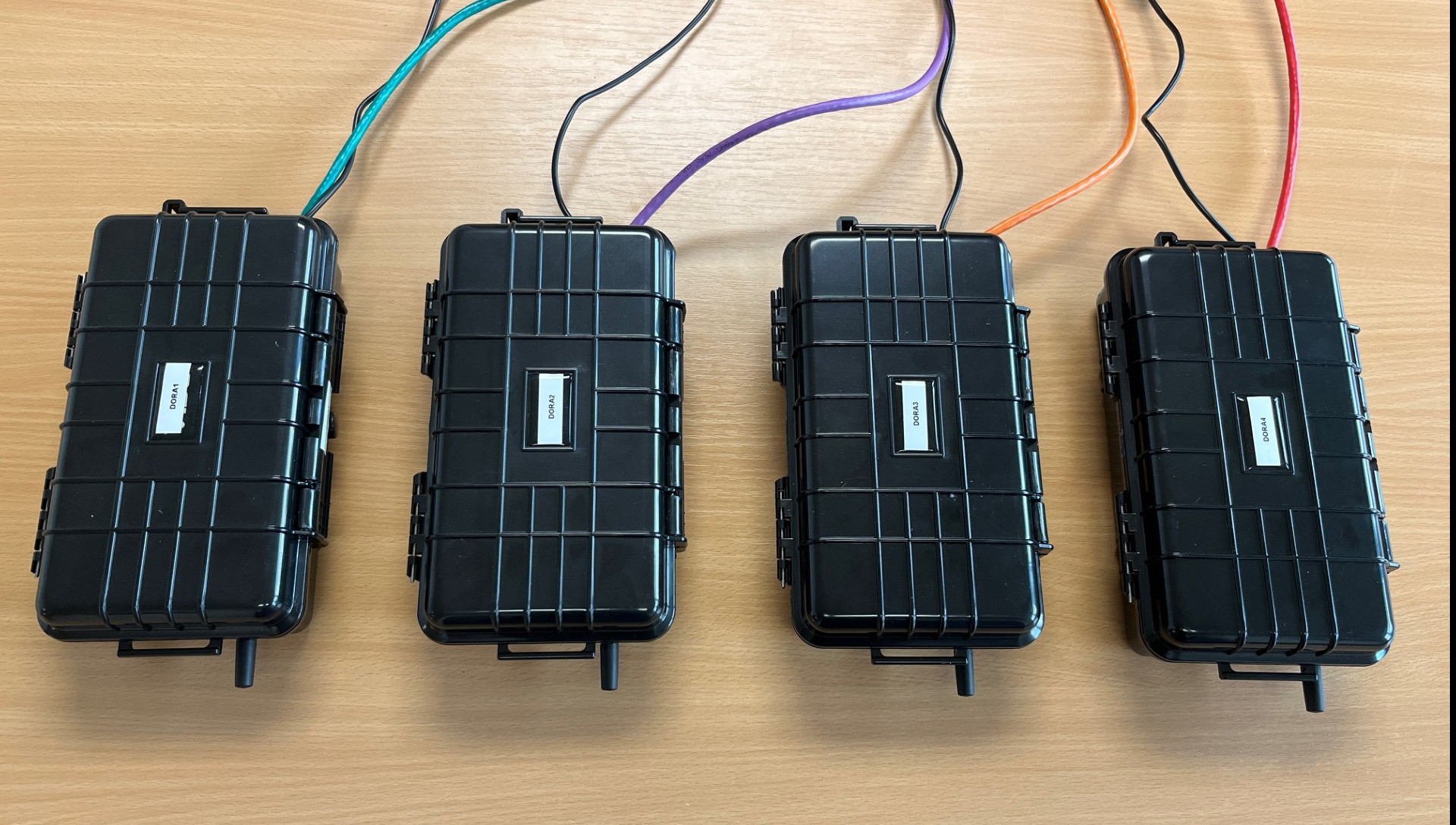
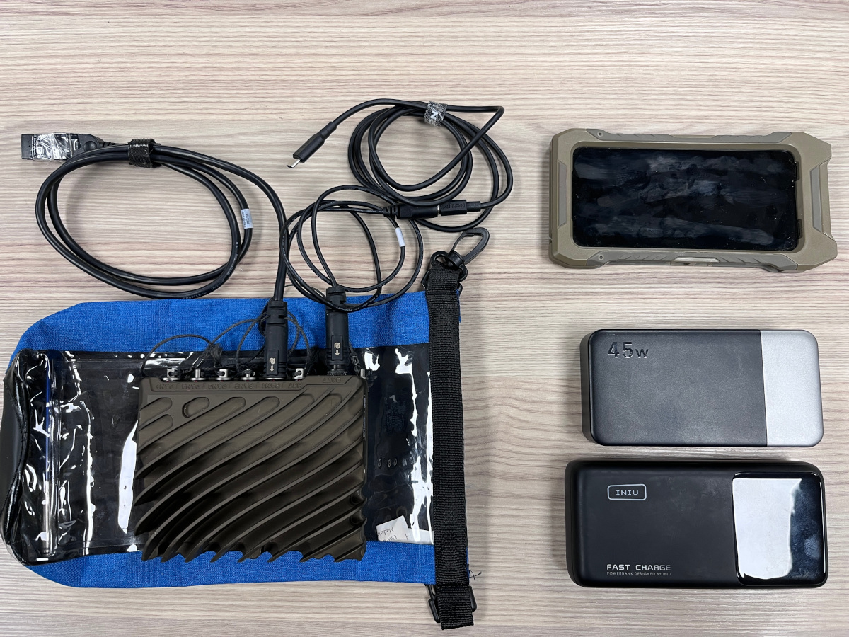
The edge compute used was a Nvidia Jetson NX 16GB onboard a Cardshark rugged computer with an external Wi-Fi adaptor to provide an access point for the phone client.
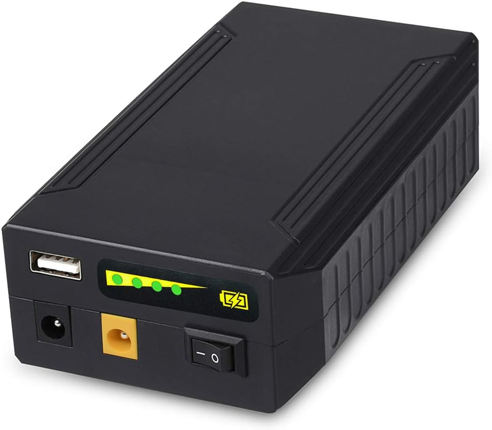
The computer was powered by budget USB-C powerbanks rated at 13000mAh and 25000mAh respectively.
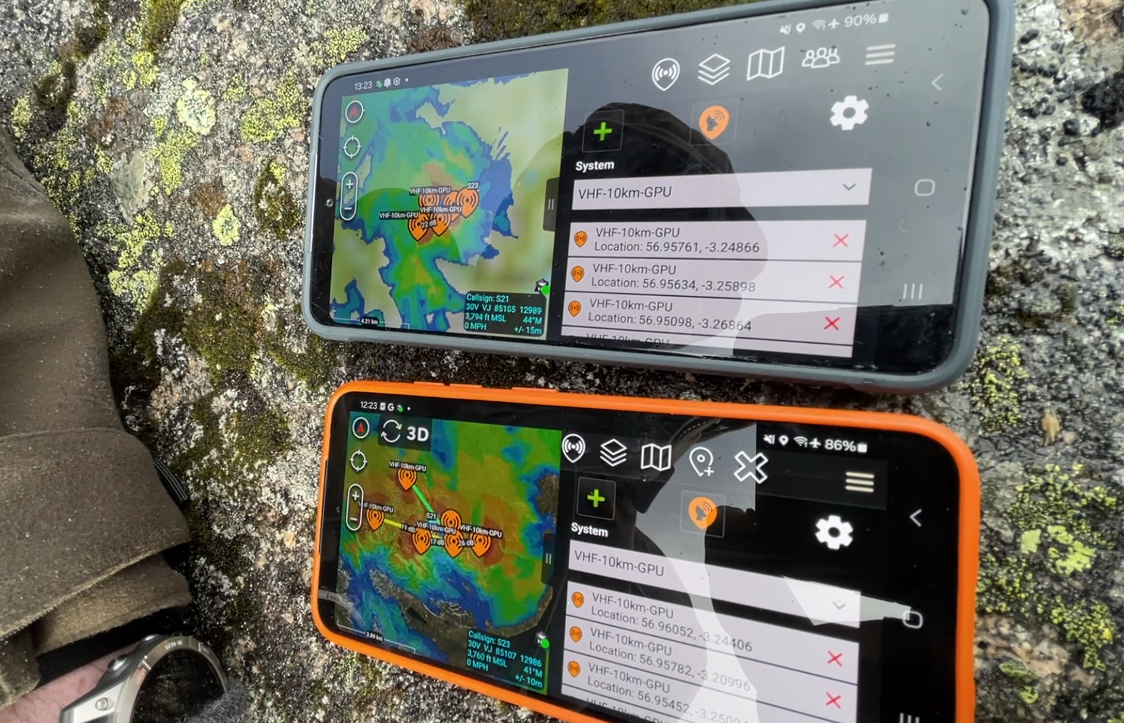
The test phone was a Samsung Galaxy S23 connected via the Jetson’s Wi-Fi.
Software
The offline software running on the Jetson’s Jetpack 6.1 OS was SOOTHSAYER v1.10, deployed as Docker containers. The resource intensive 3D engine container was not needed here so was disabled.
Services for a CoT simulator, a low power 5GHz Wi-Fi access point and a performance logging utility were running.
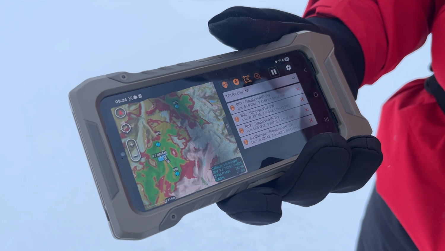
On the phone we ran ATAK 5.6.0.12 (Play store) with our SOOTHSAYER ATAK plugin version 2.7a.
Reference data
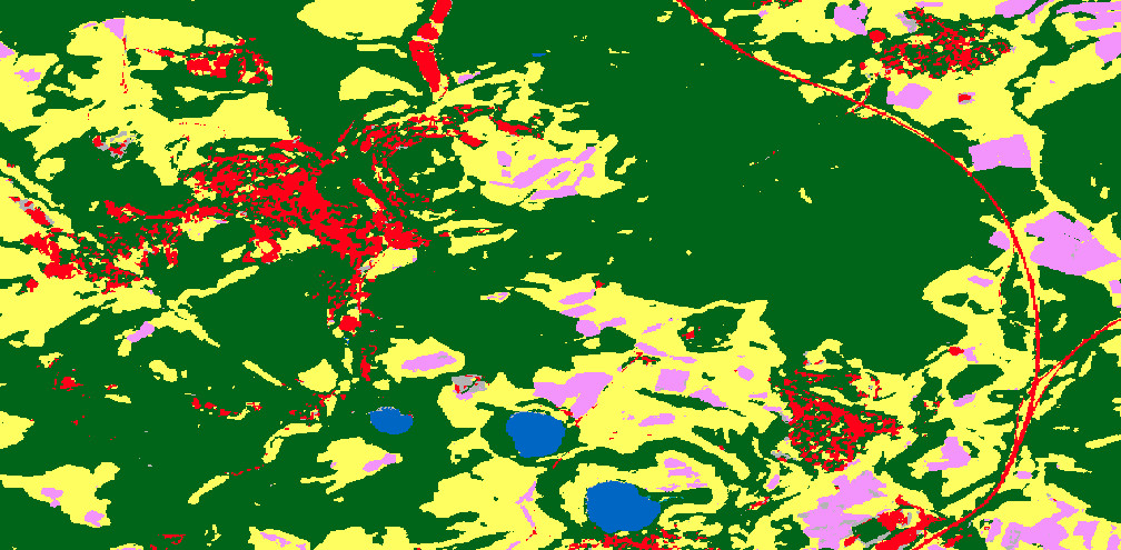
The Jetson was pre-loaded with 30m SRTM1 DTM and 10m ESA Land cover data for the mountainous test area. The phone used cached Openstreetmap mapping and 30m SRTM1 terrain data.
Test route
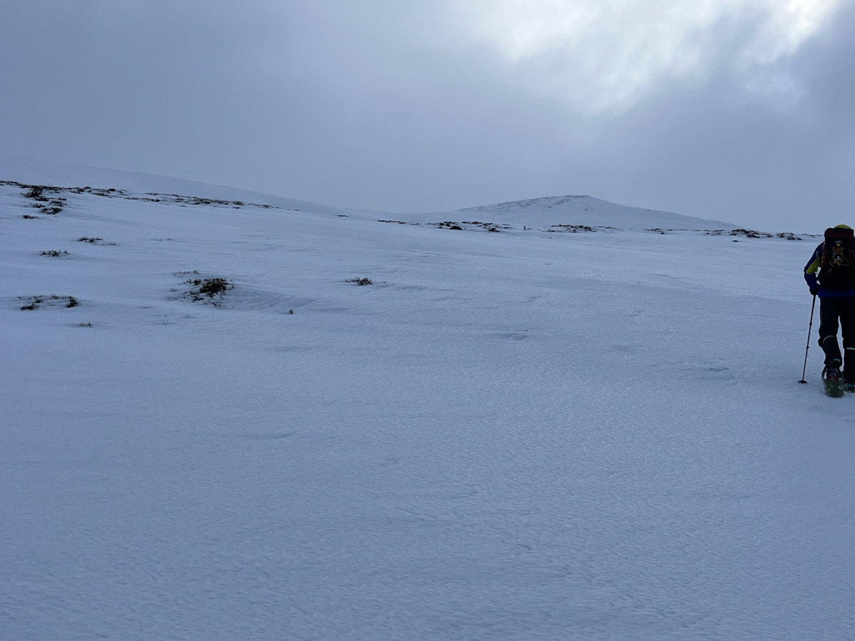
The area chosen was the Glenshee ski resort in the Cairgngorms national park, Scotland during early February where temperatures up the mountain were -10°C (14°F). A 16km circular route was followed which provided challenging conditions to meet the objectives.
Test data
Using the onboard Tegrastats utility we collected detailed data about workload, temperature and power consumption which will inform future designs and recommendations.
The day was split between two test profiles for the morning (0900 to 1300) and the afternoon (1345 to 1600).
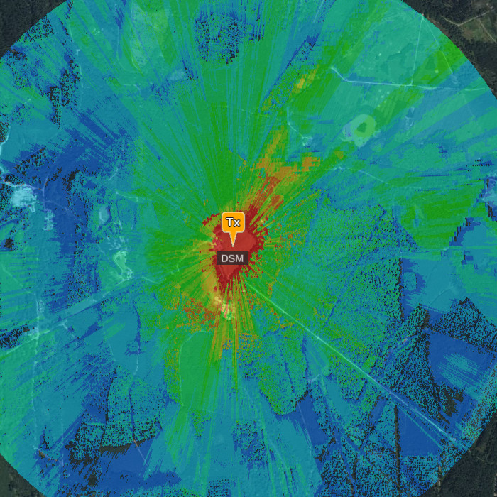
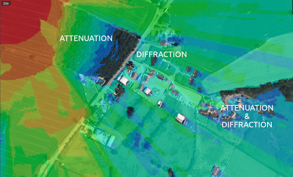
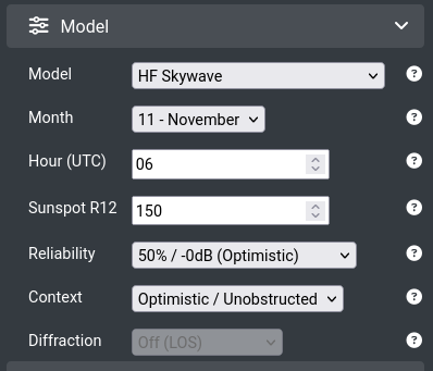
Each profile used 0.5 megapixel resolution which for a multi-site request with 5 nodes would require the analysis of 2.5 million points using the ITU-R P.1812 VHF/UHF propagation model which includes diffraction.
In the first test profile, a calculation was triggered if a radio moved more than 200m. This is an economical way of working designed to extend battery life and reduce bandwidth if working across a network.
In the second test profile, a calculation was triggered on a 10 second interval. This is a more intensive way of working which provides regular updates.
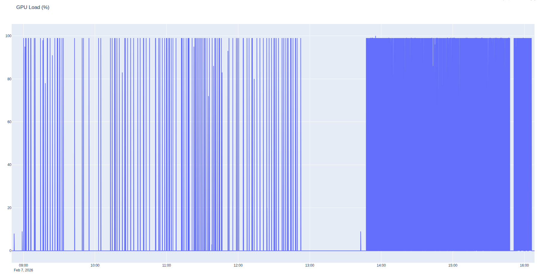
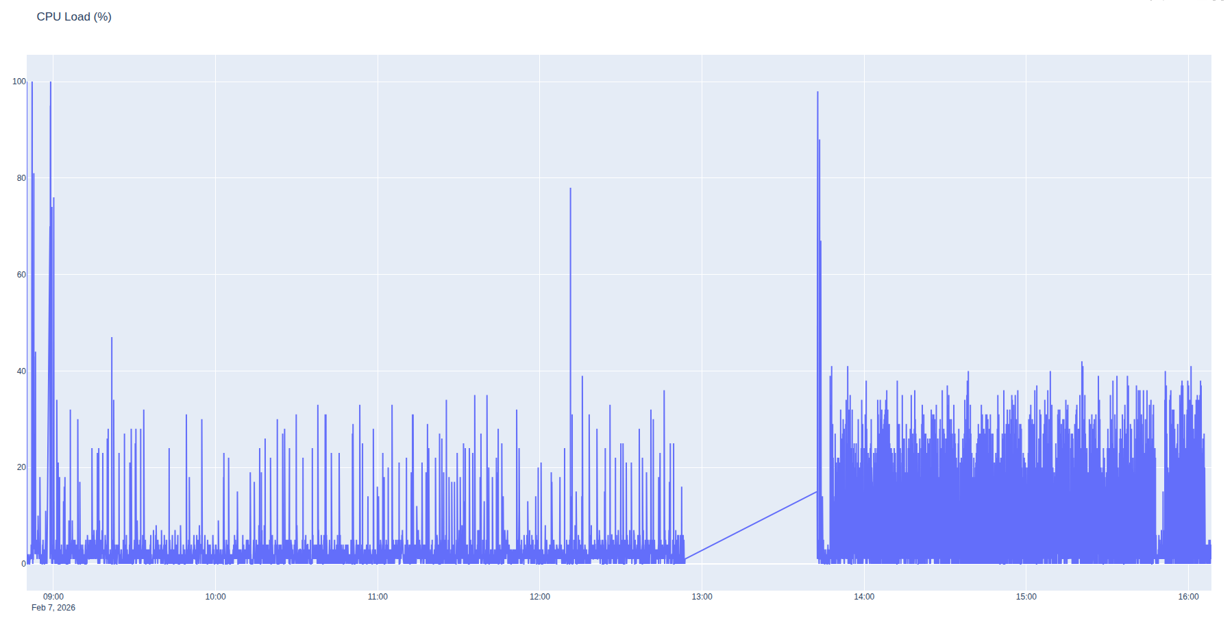
Processor load
As expected, the CPU and GPU load was more intense for the fixed interval than the responsive profile. The spacing during the responsive profile in the morning shows our slower progress on the ascent followed by rapid progress as we moved across the plateau and the server worked harder to keep up with us.
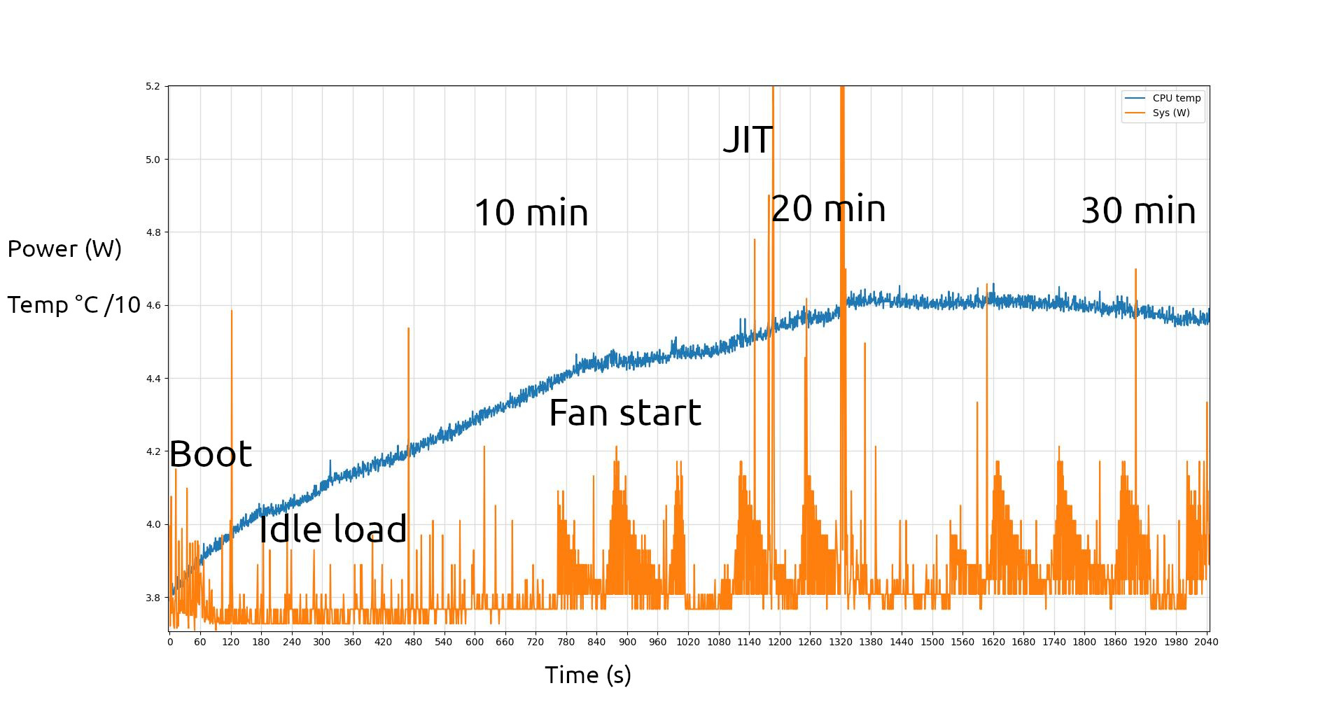
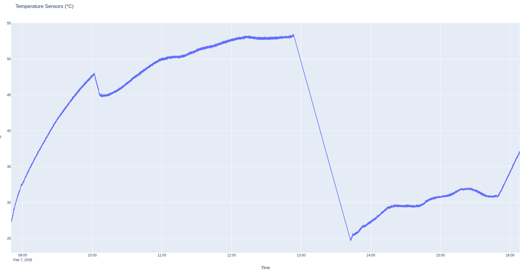
SOC Temperature
The internal SOC temperature chart was also predictable as the unit was inside a waterproof bag inside a rucksack. It climbed steadily during the ascent, then dropped sharply as we stopped to make a video where it was removed from the rucksack briefly.
The unit temperature leveled out at 53 degrees Celsius inside the rucksack. It was not an ideal place to achieve cooling but given the winter conditions, quite acceptable judging by the data. A temperature of 80 degrees would be hot.
In the afternoon the unit was attached outside the rucksack in the waterproof bag where it leveled out at 32 degrees Celsius. The moment the rucksack was placed inside the vehicle before 1600 is evident as the temperature climbed steadily. This coincided with it being placed under an intense load during a driving demonstration we have published on our Youtube channel.
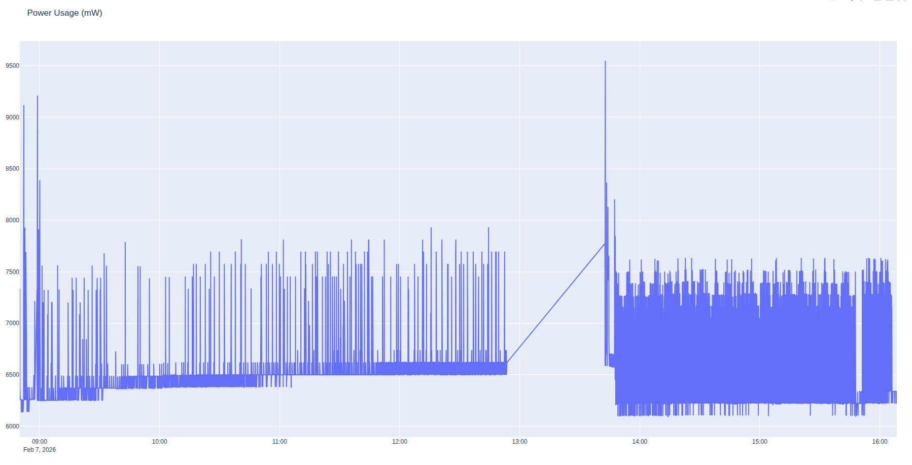
Power consumption
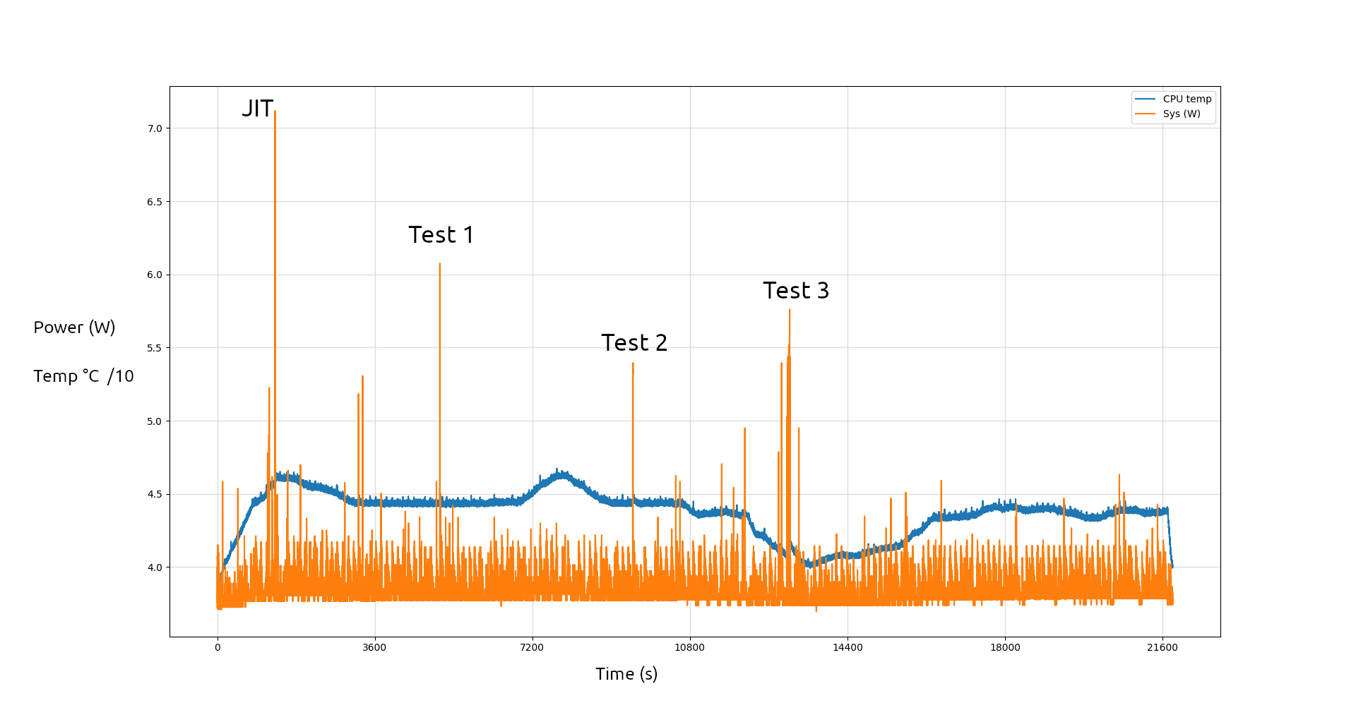
The most valuable data was power consumption which showed some interesting features and very encouraging mean values. The afternoon profile was more intense but did not increase peak power consumption which was actually lower than the morning for reasons which were not immediately obvious.
Following inspection of memory consumption (~25%), the reason was assessed to be a GPU memory leak triggered by unplanned “Above Sea Level” (ASL) calculations which occurred on the ascent. A large calculation needs more memory, which draws more power. Unlike the CPU engine which is called on-demand, the GPU engine runs continuously and its memory consumption can grow with use. In this case power consumption grew by 250mW whilst delivering 925 heat maps which we’re happy with.
The afternoon was not affected by the ASL memory leak so we maintained a steady even profile at around 7.5W power consumption, well within the range of a phone power bank.
Test videos
A video of select moments from the edge compute field test has been published on our Youtube channel. Following the field test, we created a bonus video of the drive home as the server was still running in the vehicle. This second video demonstrates the Co-Opt feature running with a 5 second refresh on a vehicle moving at up to 50 mph.
Issues
Plugin altitude logic
During the ascent we noted our own position marker, sourced from GPS, jumped from Above-Ground-Level (AGL) defined within our template to Above-Sea-Level (ASL). This was due to logic inside our plugin designed to handle aircraft.
The logic compares reported (GPS) altitude, measured in WGS-84 Height Above Ellipsoid (HAE), which is known to be inaccurate, with (ATAK) terrain height and if the difference exceeds 120m / 400ft, it uses ASL units and overrides the template’s receiver altitude to the local terrain altitude.
For more information on Height Above Ellipsoid see this article.
// If Height AGL is > 120m / 400ft, this is probably flying so we switch units to meters AMSL and use GPS altitude

if (altitude - terrain > 120.0) {

  marker.markerDetails.transmitter?.alt = altitude.toDouble()

  marker.markerDetails.receiver.alt = terrain + 1

  marker.markerDetails.output.units = "m_amsl"

} else {

  marker.markerDetails.output.units = "m"

}
This risky logic made sense from the comfort of the office with a GPS simulator but was a mess on the mountain with real GPS altitudes. The synthetic CoT markers were unaffected as they report a height above ground level.
As we went on to find, we were comparing an inaccurate GPS altitude with an inaccurate terrain altitude. Not exactly a recipe for success :/
ATAK API inconsistencies
Whilst on the mountain we noted a disagreement between our GPS altitude and ATAK’s reported altitude which warranted a deeper investigation. During the investigation we discovered inconsistencies with ATAK Elevation data.
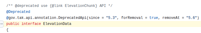
The ElevationData class we, and no doubt other developers, were using was deprecated and apparently removed in 5.6 despite being in the Hello World demo for that release. We were using this with the getElevation() method which returns the height in meters above the WGS-84 ellipsoid (HAE).
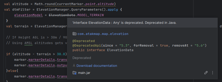
val dtmFilter = ElevationManager.QueryParameters().apply {

  elevationModel = ElevationData.MODEL_TERRAIN

}
val terrain = ElevationManager.getElevation(currentMarker.point.latitude, currentMarker.point.longitude, dtmFilter)
The recommended replacement for ElevationData based upon public source code for 5.5 is the ElevationChunk API. There are no public examples for implementing the recommended alternative at the time of writing although references were noted in documentation before it was deprecated in 5.3 which needs clarification.

DTED or SRTM?
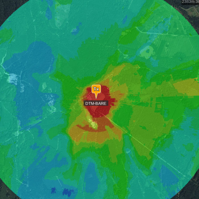
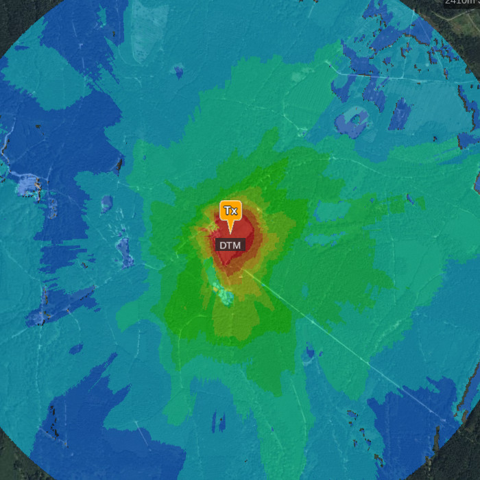
The deprecated method used was evidently returning a value based upon low resolution DTED0 data at 1km resolution. This was less accurate than the 30m SRTM1 (DTED2) data which ATAK tools like the range-bearing elevation profile or cross marker (X) use. SOOTHSAYER uses SRTM1 also.
ATAK 5.6 was found to be referencing different datasets for the same position between its interface tools and programming API which was frustrating. To prove this we pulled both the raster tiles and used GDAL’s location info utility to plot the differences for the route.
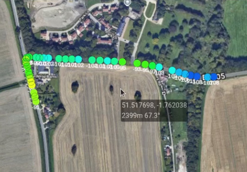
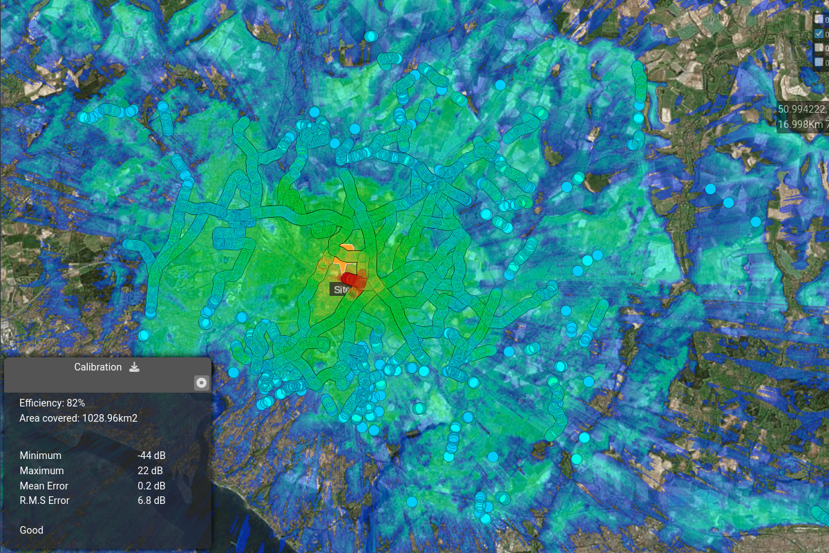
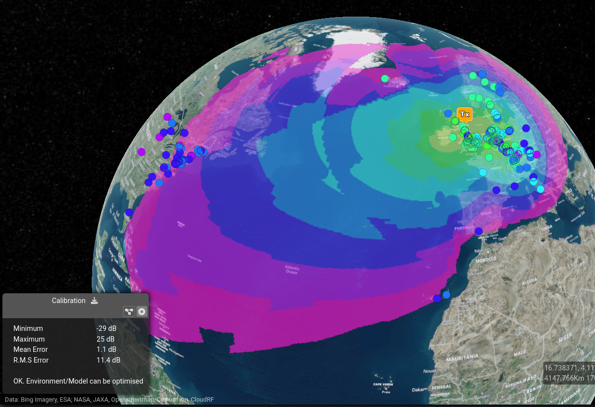
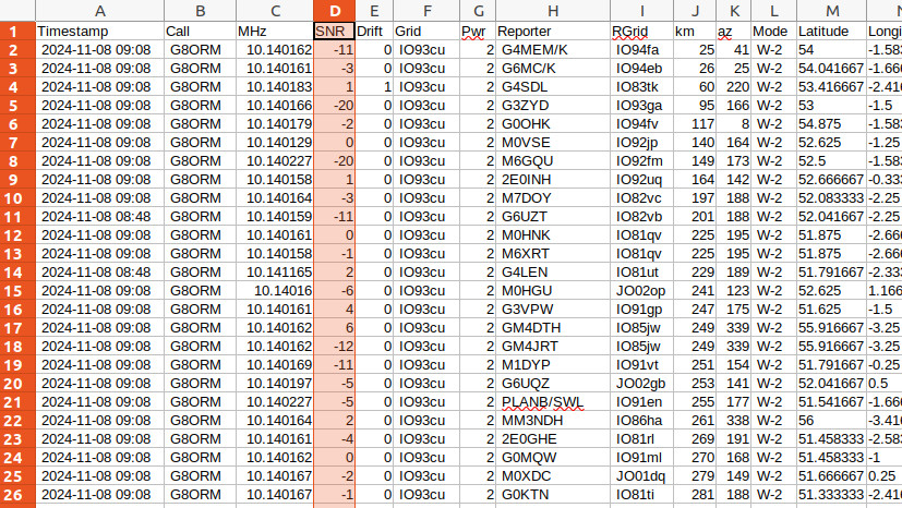
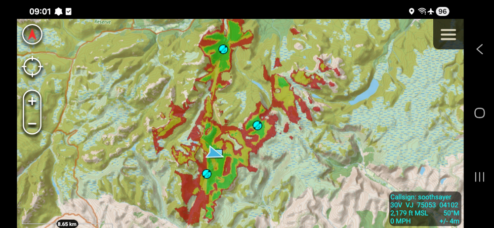
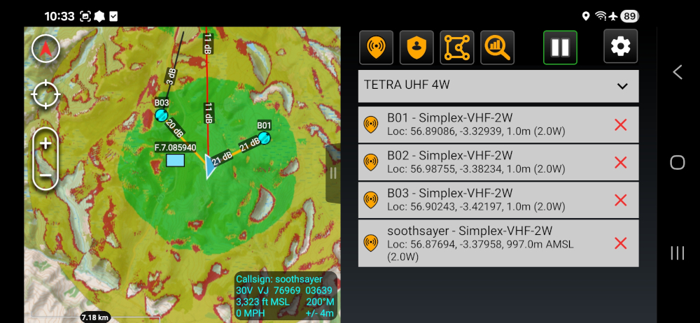
At location 56.875932, -3.377869 we experienced a large height error when the plugin fetched a height of 879m HAE yet the GPS reported 997m HAE (visible in the screenshot above). The massive 118m difference is just shy of the 120m needed to trigger our “airborne” logic.
The GPS measurement accuracy in the z-axis was measured to be inaccurate by at least 10m as the real altitude was 1007m ASL so it appears we had an altitude error greater than 120m during the ascent. A notable error which affects other GPS apps.
gdallocationinfo n56.dt0 -wgs84 -3.377869 56.875932
Report:
  Location: (37P,15L)
  Band 1:
    Value: 879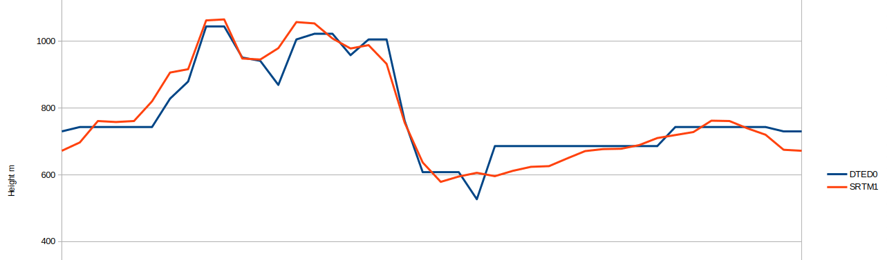
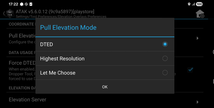
Digging into ATAK’s preferences we found validation for our theory via the “Pull Elevation Mode” option within Elevation Overlays Preferences. The choice between DTED and Highest Resolution suggests this was implemented to support better than DTED data eg. SRTM1. It is not clear if it references DTED0 or SRTM1, which as we’ve shown could be a +100m error.
Some batteries are better than others
Our goal was to use flight-safe USB power banks which can easily provide the 7-8W of power needed to run the capability. We ran soak tests in the office to establish a battery life of 6 hours for the smaller 45wH battery. We expected this to be reduced on the mountain so purchased a larger 92wH battery but it failed after 4 hours despite being kept warm inside an insulated jacket.
The smaller battery proved its worth and ran for two hours with only 35% consumption suggesting it would have lasted longer than the larger battery.
During subsequent charging of the large battery it reported unexpected levels suggesting it was likely defective and under performing.
Our conclusion was that you can live-map a network for more than four hours on a small battery, but it must be a reliable one.
Conclusion
We were happy with the test and the results which showed solid stability and good power economy. It validated the hardware, the SOOTHSAYER API and most importantly the concept of edge coverage mapping.
Given the accuracy issues experienced with GPS data and the deprecated-yet-still-going elevation APIs using low resolution data sources, we have commented out the error prone “airborne” logic in our plugin and will only use the fixed altitude(s) defined within the radio template until further notice.
Plugin users can edit both the transmit and receive altitudes above ground level by selecting the marker then clicking the pencil.
The ATAK plugin has already been updated and pushed to our Github repository and Google Play as version 2.7.1