Noise is the single biggest factor in determining the quality of a communications link. It’s also the reason why there is low confidence in the accuracy of (RF) simulation in complex environments as it’s rarely done well, if at all.
Budgeting for noise is critical to achieve desired signal levels. Historically, it was done with a single figure to satisfy all locations, eg. ‘-100dBm’. This simplification is a time/accuracy trade-off and is no longer relevant in the age of dynamic spectrum management and cognitive radio.
Noise varies widely between locations, and changes constantly, so we have invested in developing living noise maps to reflect this dynamic nature. Like a terrain layer that moves, noise data can be used to improve the accuracy and relevance of planning in dynamic environments.
Evolution of simulating noise
A noise figure (2022)
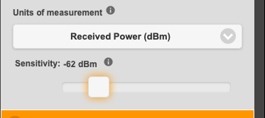
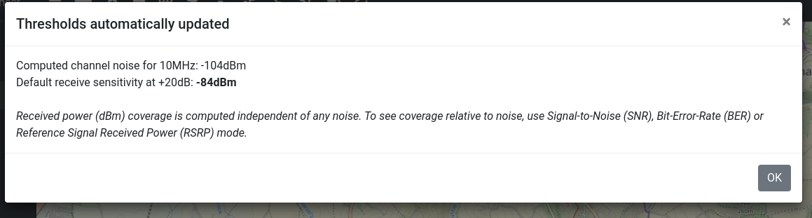
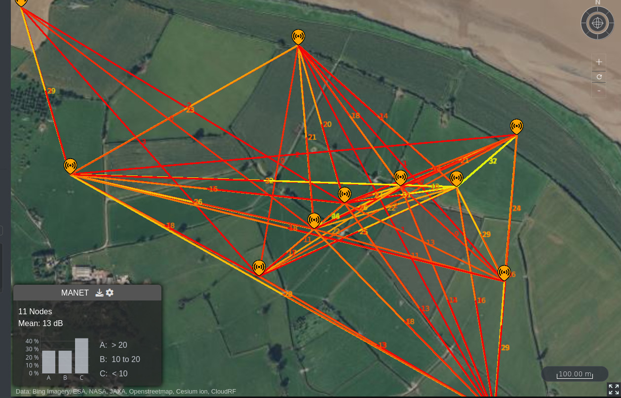
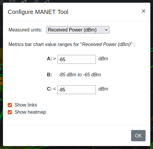
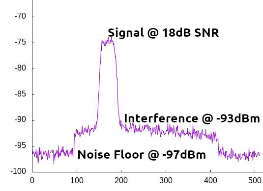
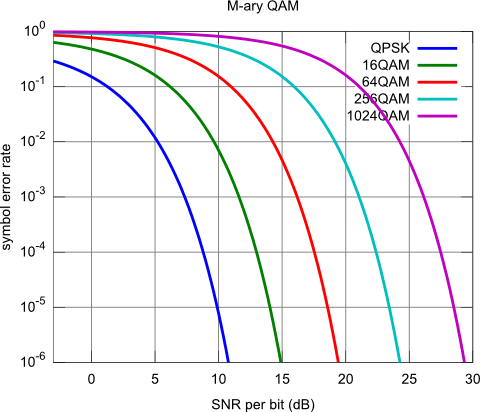
Back when we added Signal-to-Noise (SNR) output units in API v2.7, we needed to express the noise floor as a (dBm) figure to provide a reference for a signal’s quality eg. 15dB. Users interested in SNR enter a single value like -100dBm, hopefully based on the local environment, to describe noise across the entire area, or link. As this guesswork is prone to error, we automatically recommended a conservative value, to budget for high noise.
For example if the thermal noise for a narrow channel is -133dBm, our interface automatically recommends -113dBm as a floor for planning which provides 20dB for unknown noise.
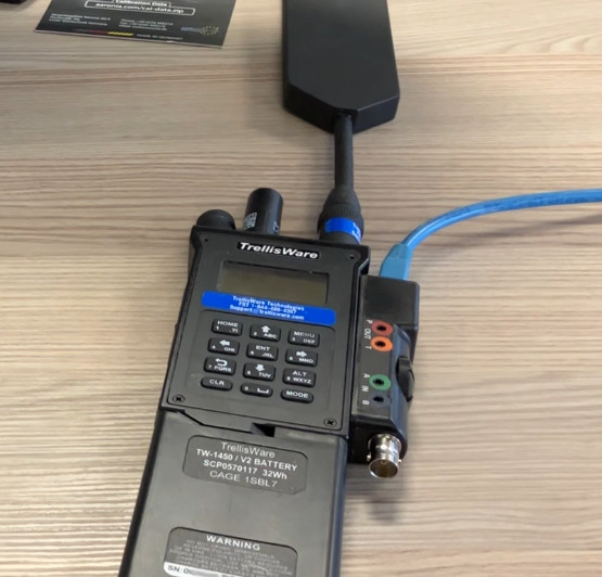
The noise figure could be measured direct from a networked sensor which we published in early 2023.
A Noise database (2023)
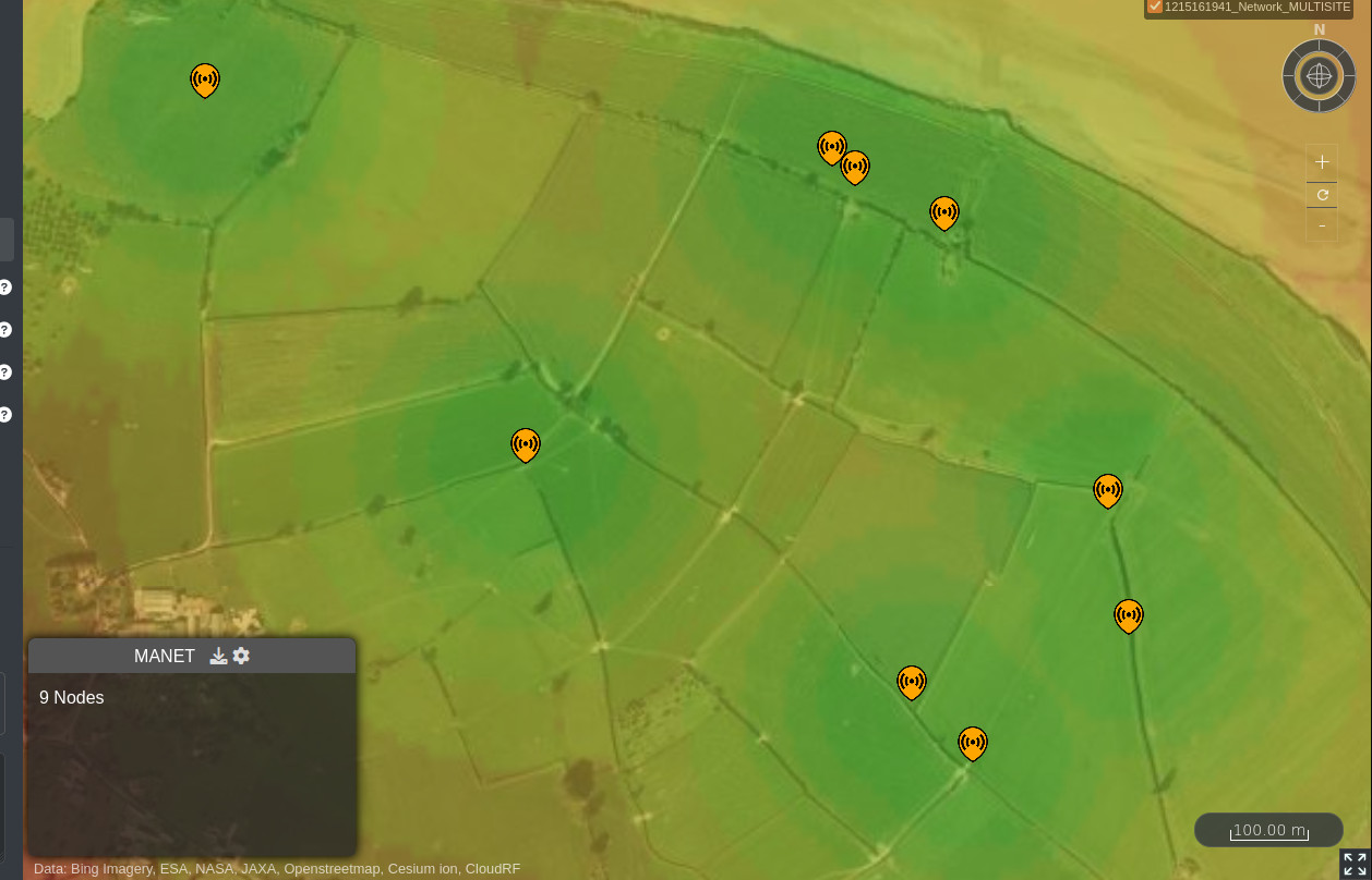
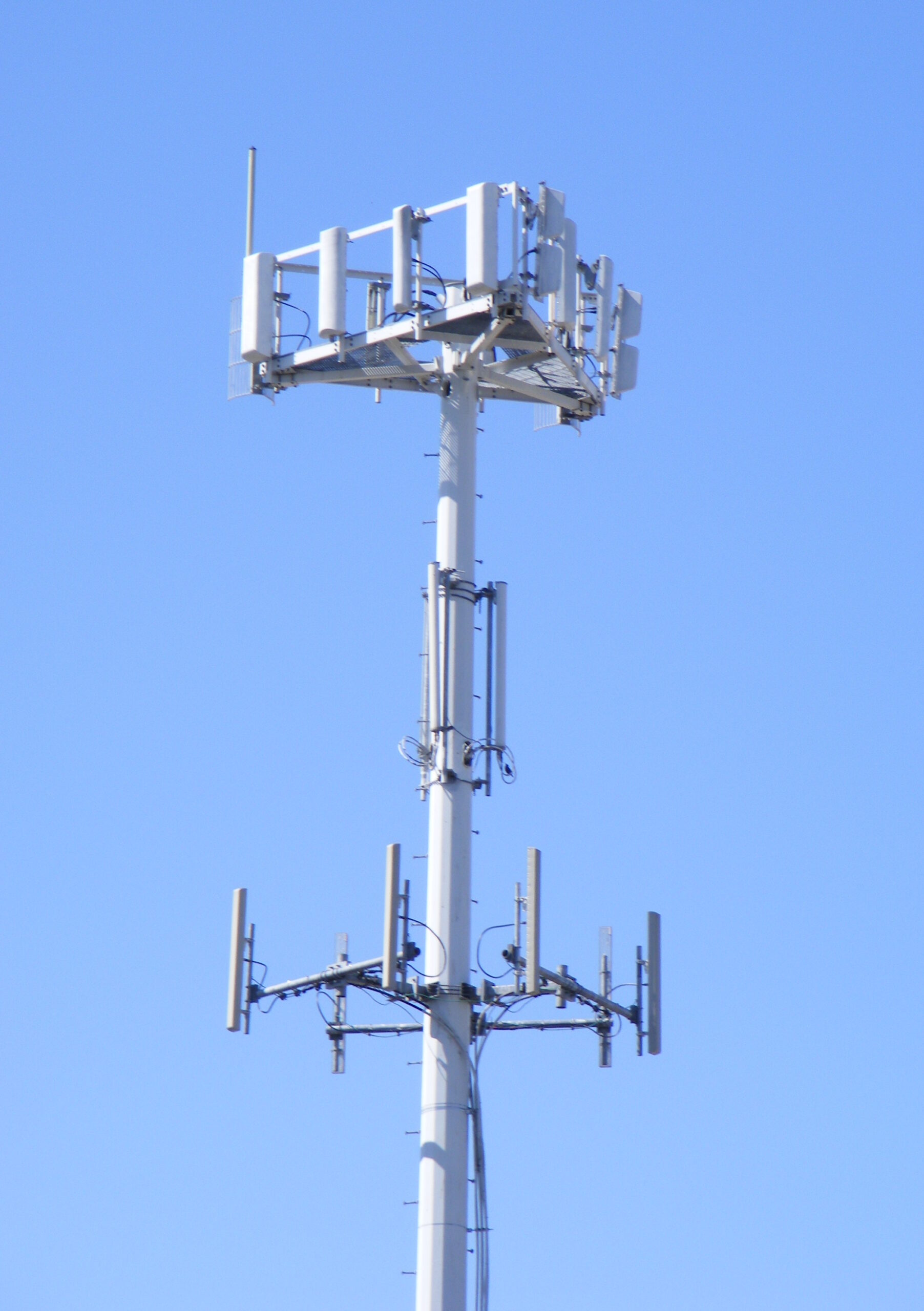
Noise varies by location (and frequency) and the previous method didn’t scale so we developed a noise API to store noise data and reference it in calculations. The private data was used on a per-site basis so you could model a network with different noise at each site. A marked improvement on a single figure.
This development represented a leap forward in network planning as each node could be configured for the local environment, which can vary drastically. Two different users might have different needs so it is isolated to the user’s account. A multisite API call accepts different noise values for each site.
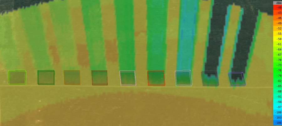
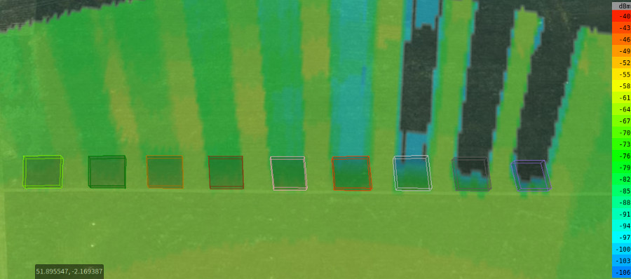
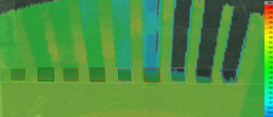
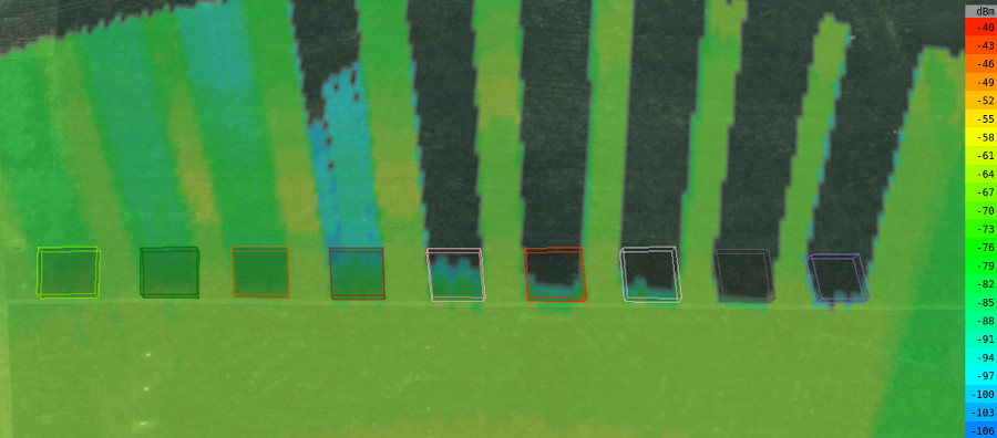
A Noise map (2025)
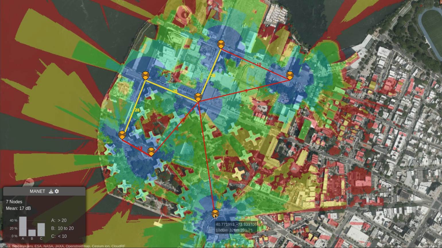
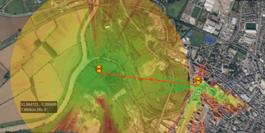
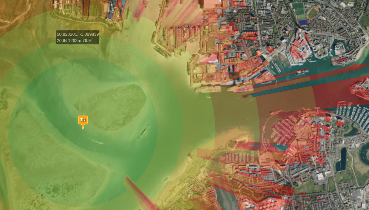
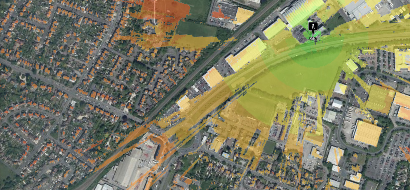
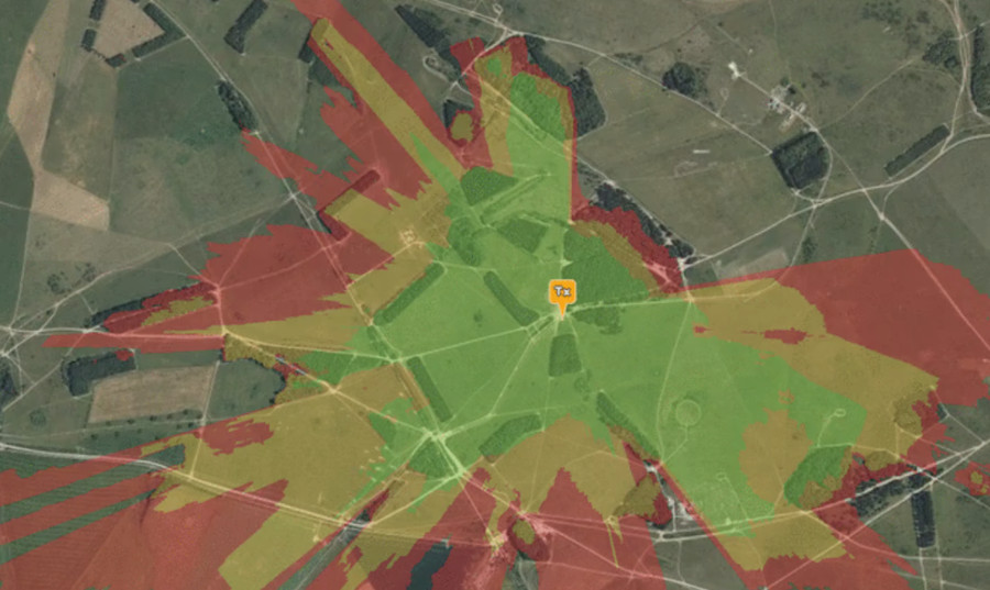
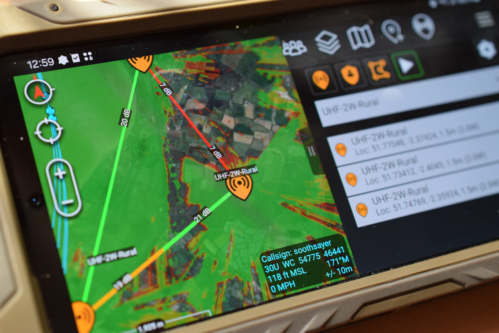
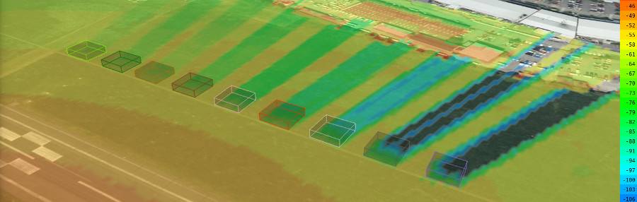
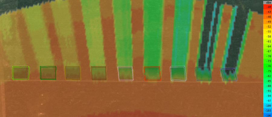
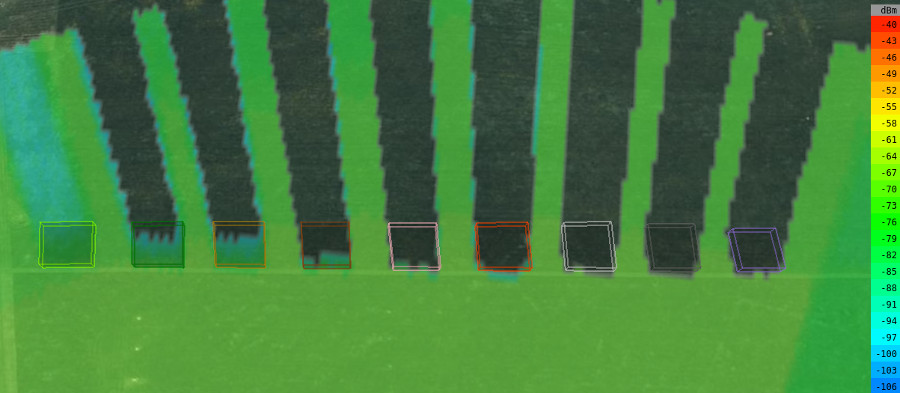
Building upon our Noise API, stored data was used to generate a noise map, specifically a raster layer of measurements, similar to clutter which our API can reference. This noise map describes thousands of noise points across the area or link of interest and provides high resolution noise. Now you can see the real impact of noise with minimal effort at each location covered.
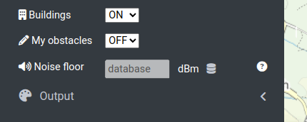
Any calculation requested with the database option versus the legacy single figure method will create and use a noise map at the API. The quality of the noise is determined by the data you can provide and any missing values will be interpolated. The maximum resolution is 12m supporting dense urban planning so you can have different noise levels in adjacent streets, which is common in urban canyons.
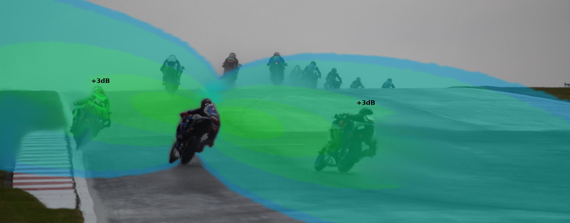
Better still, with live noise data, you get live coverage. Ideal for autonomous systems and future spectrum management systems which will need to be automated to remain relevant.
Collecting noise with DORA
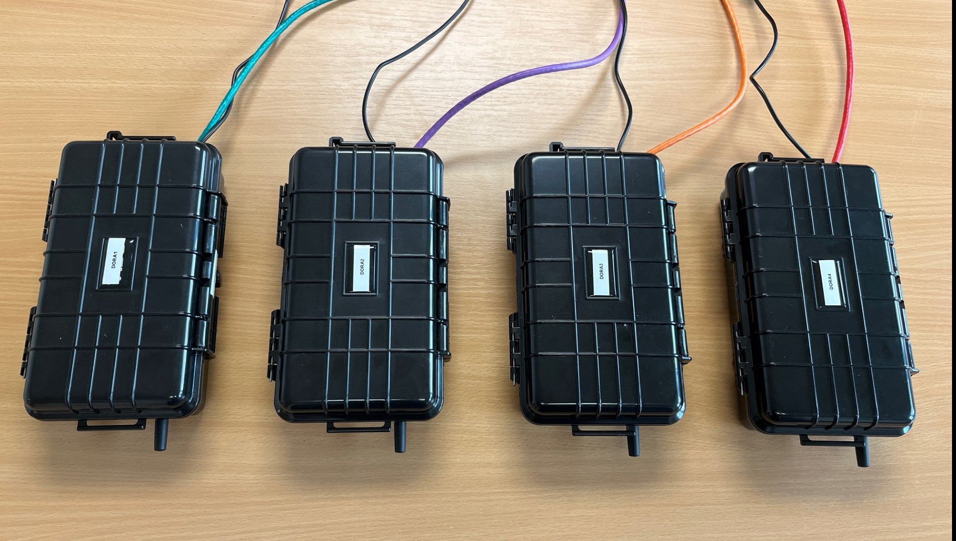
DORA (Distributed Open Receiver API) is an open source project sponsored by CloudRF designed to collect noise measurements using various Software Defined Radio (SDR) receivers and mature open source utilities.
It uses consumer grade SDRs via a remote service present on the DragonOS operating system. Designed for SBCs like Raspberry Pis, DORA presents a common API for RF sensing across different radios. Nodes perform a local FFT to measure average power (with configurable bandwidth) and then publish the PSD data via an API endpoint. A server fetches and collates these to present them in an interface to provide spectrum visibility.
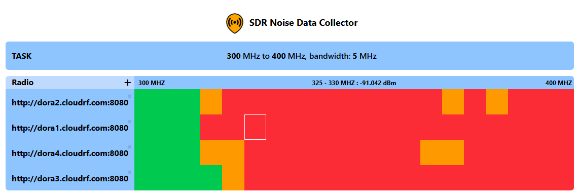
When a CloudRF API key is provided, the server sends data to our noise API giving a user live noise data for accurate planning. DORA’s low cost (£200 BOM per node) makes it scalable and cost effective. It won’t give you a pretty waterfall like Government spec hardware but it will provide the scale needed for autonomous spectrum management, powered by the CloudRF API.
If you do want an open source FFT and waterfall we recommend OpenWebRx.
You can contribute to the future of scalable spectrum sensing over on Github with issues, feedback and features.
Summary
This noise map feature is live now and works with any receiver capable of reporting noise as dBm. The benefit of using live noise in planning is improved accuracy but also relevance, and in time confidence, as the simulation will match the environment.


 Jamming is a form of electronic attack which uses a stronger signal to disrupt target wireless devices.
DISCLAIMER: It is an offence to intentionally interfere with someone else’s use of the wireless spectrum in the UK.
The mention of its name also disrupts rational thinking amongst otherwise intelligent people and its common for spectrum planners and event managers to ignore signal theory when discussing its impact and revert to hollywood instead.
Originally used in warfare, it’s now commonly used in civil emergencies such as event protection, bomb disposal or hostage negotiation.
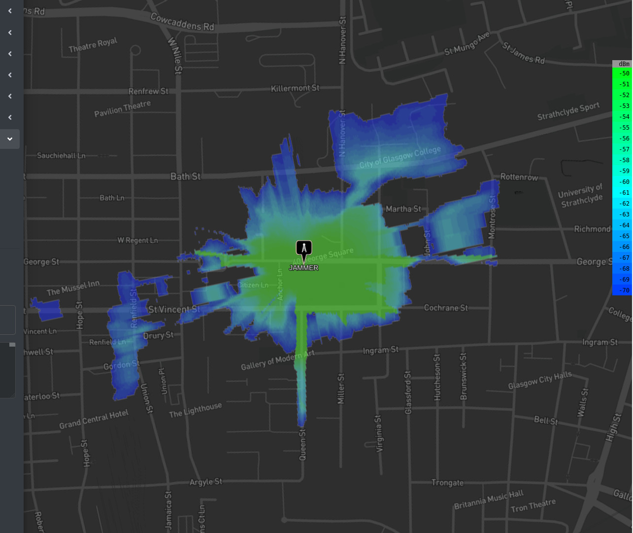
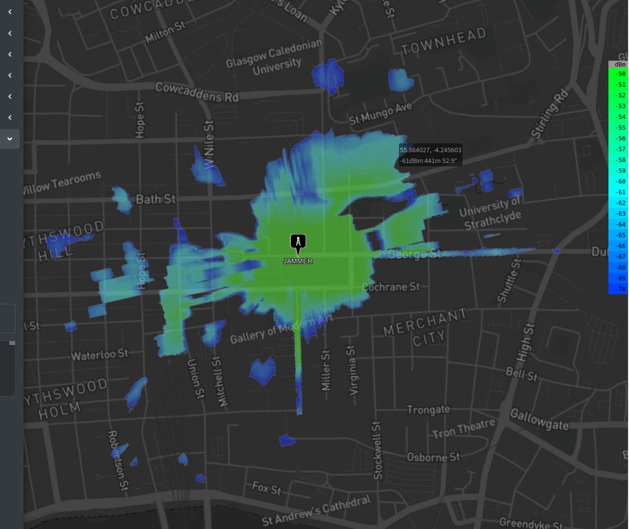
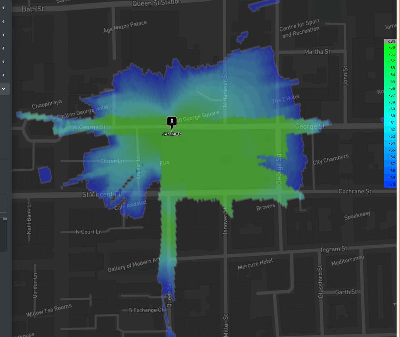
This blog uses modelling evidence to demonstrate the impact of jamming in a city and in the process, debunk popular jamming myths. The target band in all models is the 2.4GHz ISM band which is easily the busiest unlicensed band in the world and home to WiFi, Bluetooth, CCTV, Locks, Sensors, Drones and phones. The chosen location is George Square in Glasgow which is a large open surrounded by tall stone buildings. The antenna used is Omni-directional to visualise the effect in all directions.
Jamming is a form of electronic attack which uses a stronger signal to disrupt target wireless devices.
DISCLAIMER: It is an offence to intentionally interfere with someone else’s use of the wireless spectrum in the UK.
The mention of its name also disrupts rational thinking amongst otherwise intelligent people and its common for spectrum planners and event managers to ignore signal theory when discussing its impact and revert to hollywood instead.
Originally used in warfare, it’s now commonly used in civil emergencies such as event protection, bomb disposal or hostage negotiation.
This blog uses modelling evidence to demonstrate the impact of jamming in a city and in the process, debunk popular jamming myths. The target band in all models is the 2.4GHz ISM band which is easily the busiest unlicensed band in the world and home to WiFi, Bluetooth, CCTV, Locks, Sensors, Drones and phones. The chosen location is George Square in Glasgow which is a large open surrounded by tall stone buildings. The antenna used is Omni-directional to visualise the effect in all directions.