Antennas Archives

Posted on 2024-01-082024-01-08

HF Near Vertical Incidence Skywave (NVIS)

Today we launched a new model for ionospheric communication planning with High Frequency Near Vertical Incidence Skywave (NVIS).

It’s available in the interface and directly via the area, path, points or multisite API calls. The powerful GPU accelerated capability offers a modern way of visualising and teaching NVIS propagation. It does not, in it’s present form, do frequency selection so this must be performed prior to using this tool to visualise the coverage.

Background

This form of basic ionospheric propagation is popular with Military, Maritime and rural customers. With a simple horizontally polarised antenna and the right frequency, an operator can establish a link of up to 500km making this a quick and economical method for communicating long distances.

HF is undergoing a renaissance driven by uncertainty of the availability of space systems and the need for secondary communications in emergency PACE planning. Despite the choice available now with consumer grade space based communications, HF is a low cost method which requires no third parties making it immune to business and geo-political changes.

As HF bandwidth is very limited, historically only CW and voice channels were viable although developments in compression, cognitive radio and now MIMO are changing this. Improvements in software especially mean that reliable data channels with improved throughput are possible which makes HF data links a popular low cost, low bandwidth, alternative to satellite communications.

Ionospheric propagation

The ionosphere describes layers of ionised gas between earth and space which vary in height between around 100 and 300km. These layers reflect (HF) radio waves and attenuate others. As the layers are stimulated by sunlight, propagation changes significantly between day and night. Seasons affect propagation also, so a frequency which is good in the day may become unworkable after sunset.

The D Layer is the lowest layer at around 100km and absorbs low frequencies (2-4MHz). This weakens at night so these frequencies become viable. This determines the Lowest Usable Frequency (LUF).

The F layer is the highest layer at around 300km and reflects higher frequencies between 4 and 8MHz. The critical frequency is the Maximum Usable Frequency (MUF) which changes throughout the day, determined by sunlight.

A useful analogy for considering the change in the layers is a car engine; It warms up quickly in the morning and cools gradually at the end of a day driving. HF layers change quickly at dawn and slowly after sunset.

Higher frequencies beyond 8MHz experience less refraction so pass through the layers out into space. Depending on conditions a higher frequency may be possible but the most reliable (for NVIS) are found between 2 and 8MHz.

Using the NVIS model

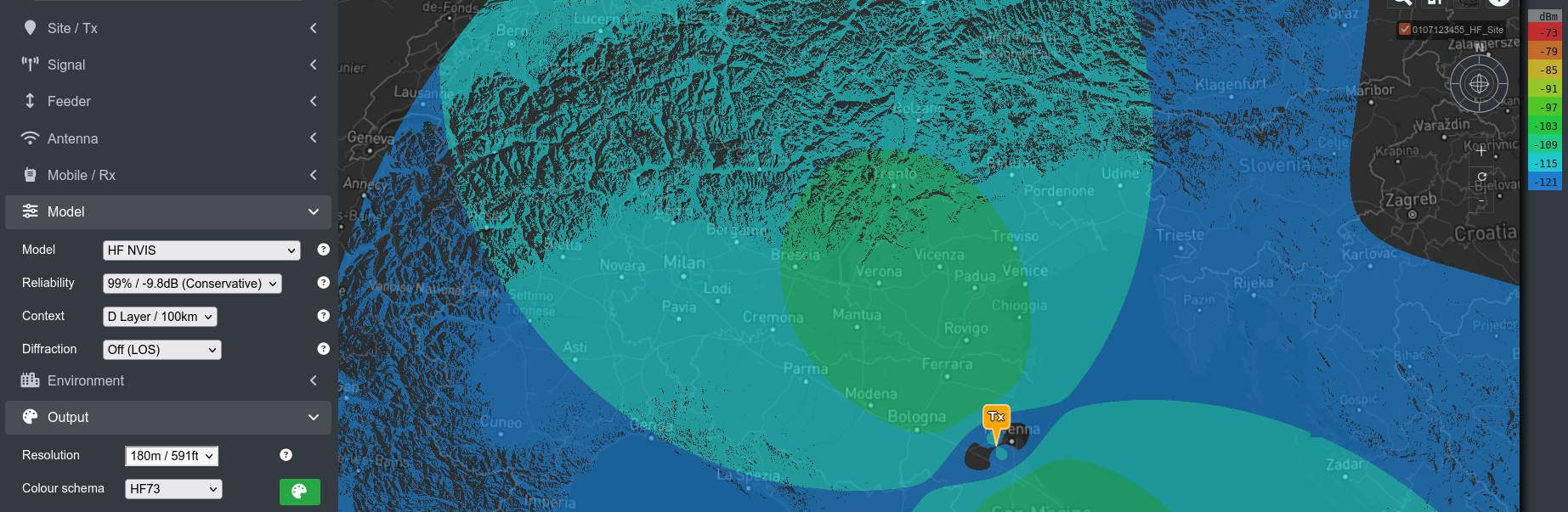
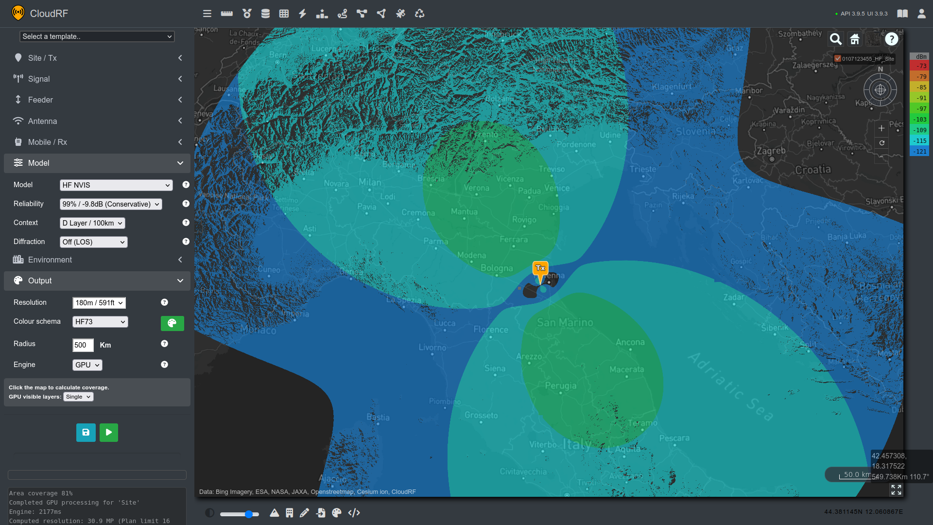
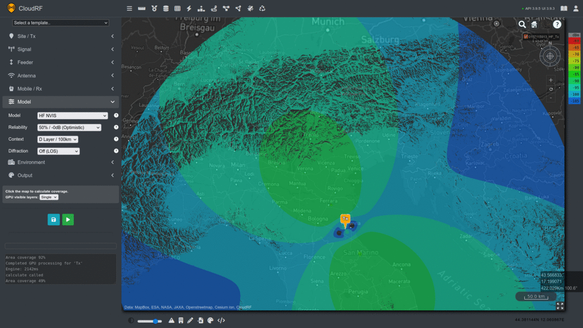
The HF NVIS model can be selected in the model menu or in the API as code 12. Like other models it has a configurable reliability (aka fade margin) and a “context”. The context here refers to the refraction altitude and not an environmental eg. urban/rural choice with other terrestrial models.

Context 1 is the D layer at 100km – (Day)
Context 2 is the E layer at 200km
Context 3 is the F layer at 300km – (Night)

In the day you should use the D layer and your frequency should be between 4 and 8 MHz.

At night, you will use the F layer and need a lower frequency between 2 and 4MHz.

This HF model is only for use with a pre-determined frequency. It does not do forecasting or LUF/MUF frequency selection. This functionality will follow.

The reliability option provides a 10dB fade margin to tune modelling to match the real world. This was set with 50% reliability aligning to summer predictions with a 5MHz frequency.

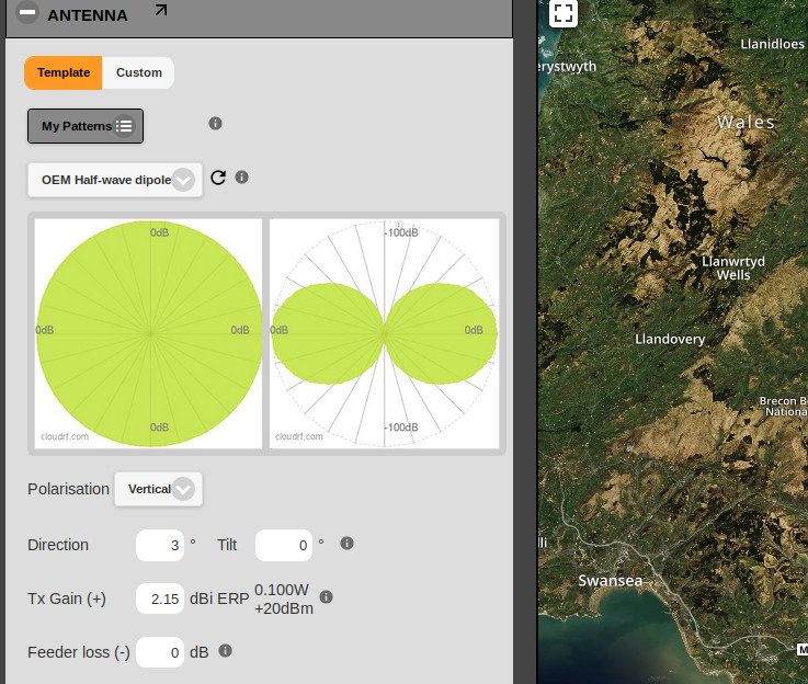
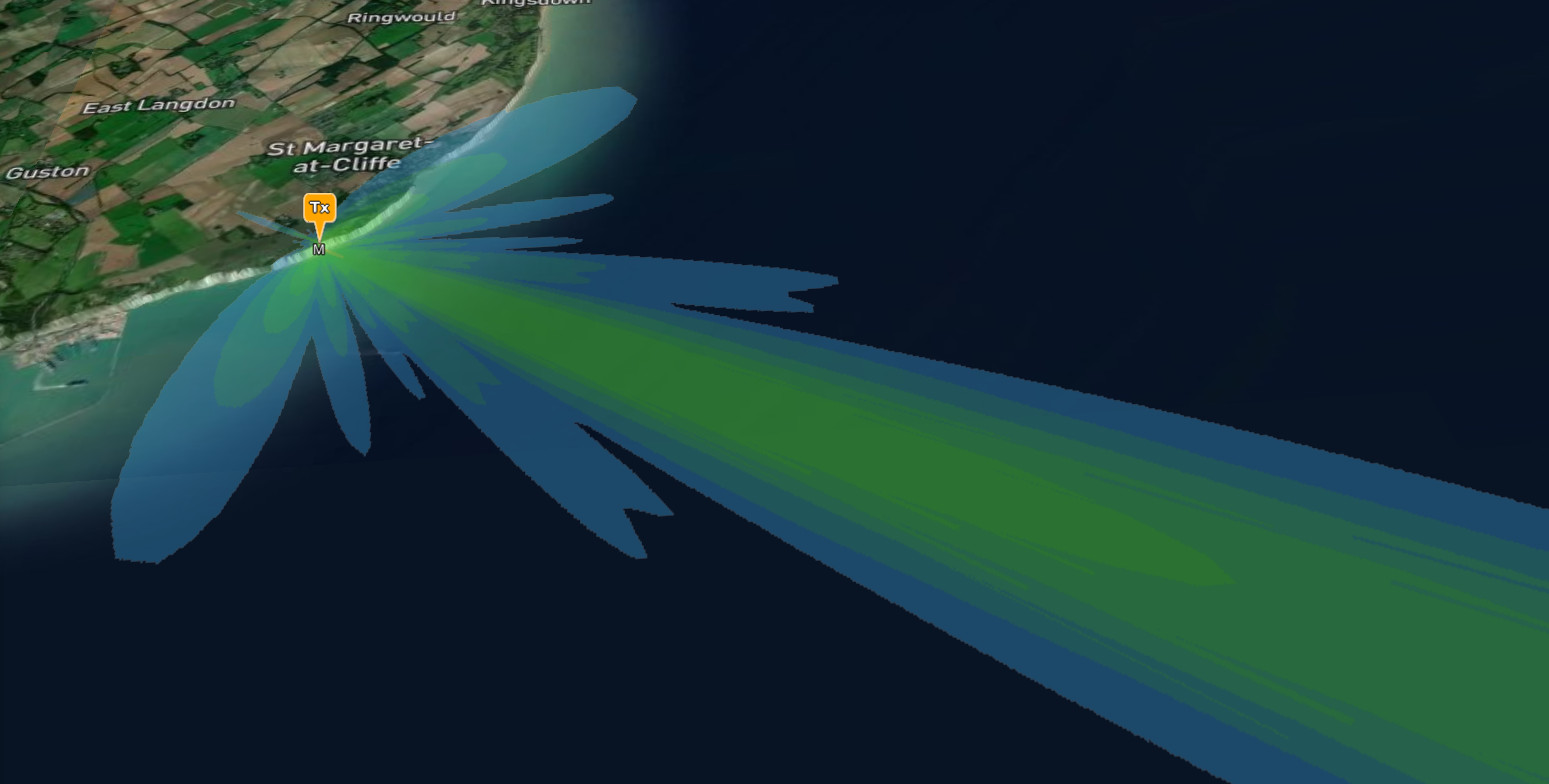
HF dipole antenna

The antenna pattern will be a special horizontal dipole. You may set the gain and azimuth only but cannot change the pattern as it has high angle nulls for the skip distance before the reflection hits the earth. This will manifest itself as a cold zone at either end of the dipole where the pattern gain is lowest.

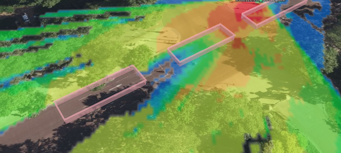
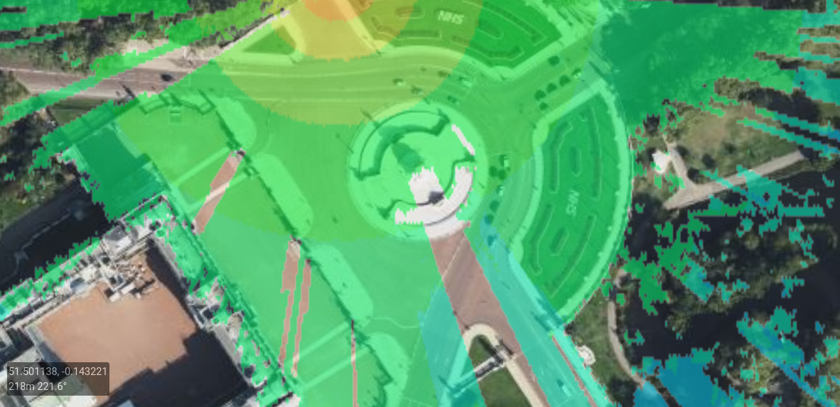
This animation shows a dipole orientated north west. The angle of orientation is measured perpendicular (at a right angle) to the wire so the tips of the antenna will generate the worst coverage, in this case to the north east and south west.

Radius and resolution

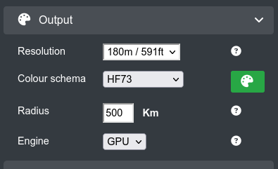
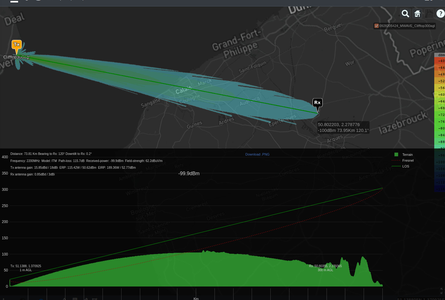
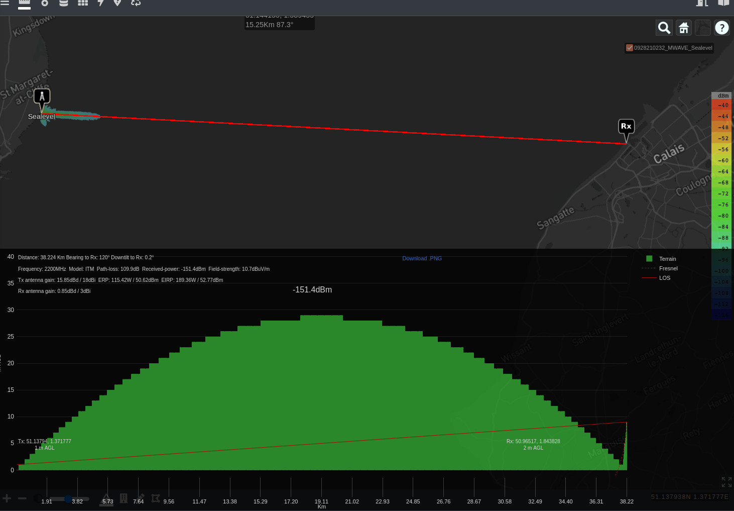
The recommended resolution for NVIS is 180m due to the immense size of the problem. Land cover is irrelevant with this mode of propagation. The radius has been limited to 500km in line with API limits. You can go further with NVIS but would run a risk of straying into multi-hop HF Skywave and this capability is focused on one hop only.

Most NVIS communication takes place between 50 and 300km where groundwave ends and the signal fades into the noise floor.

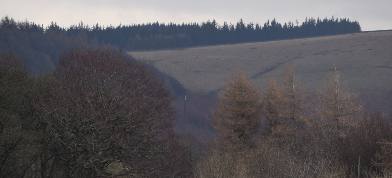
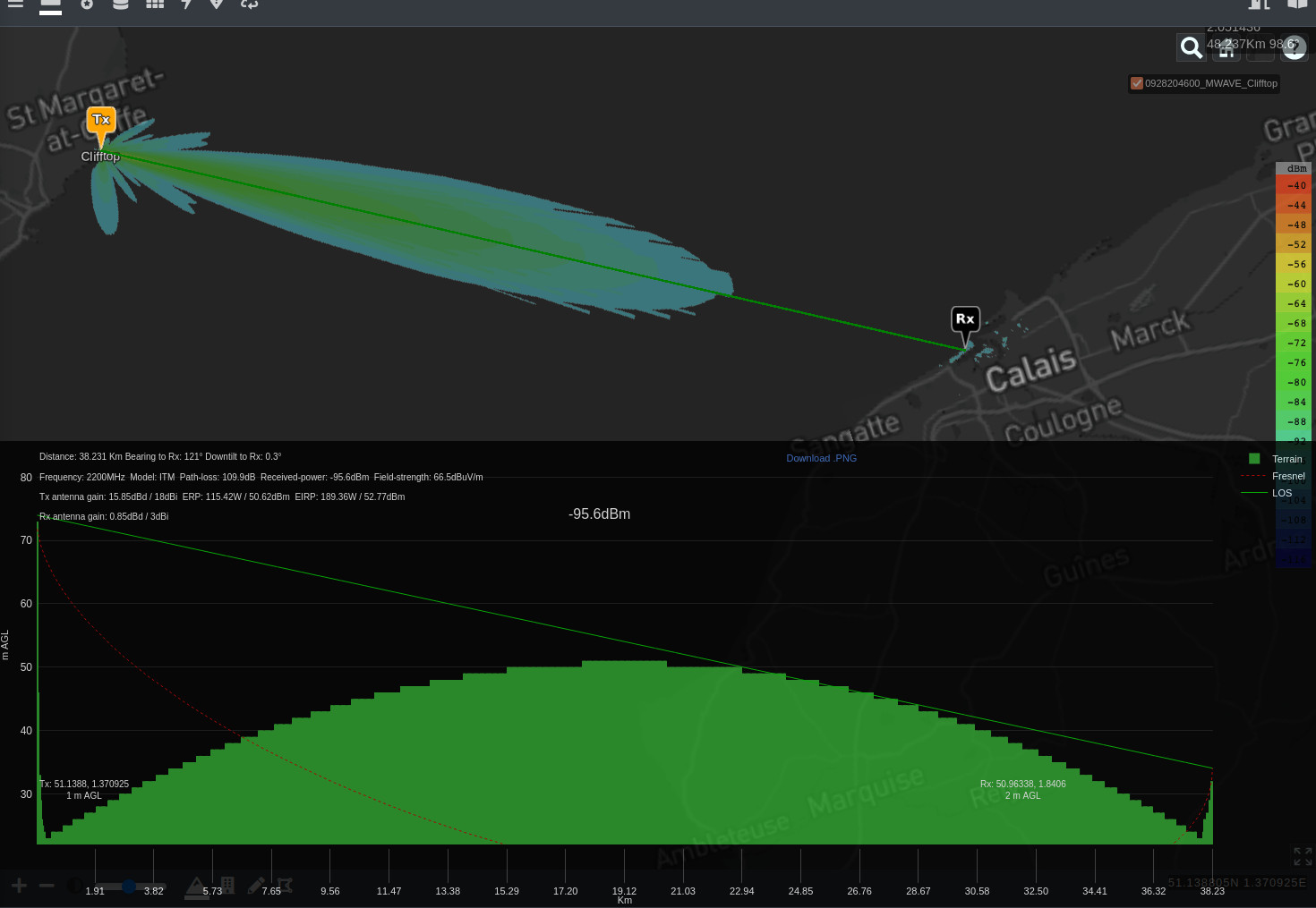
Using the GPU engine we can model a 500km radius with NVIS and terrain in under 3s. Terrain is a small concern to NVIS unless it’s a large mountain several hundred km away. In this case you will experience shadows due to to low angle of incidence but compared with shadows from terrestrial communications, it will be small.

Environment layers such as land cover and buildings should be off. They will be ignored at 180m resolution.

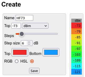
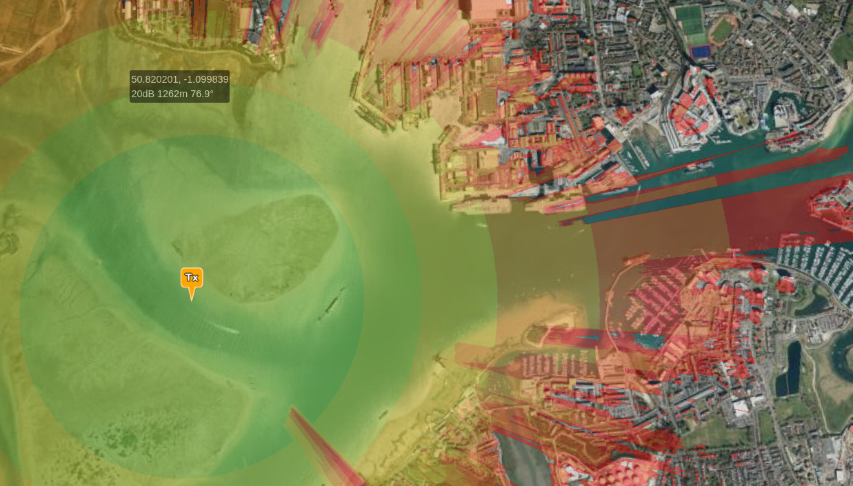
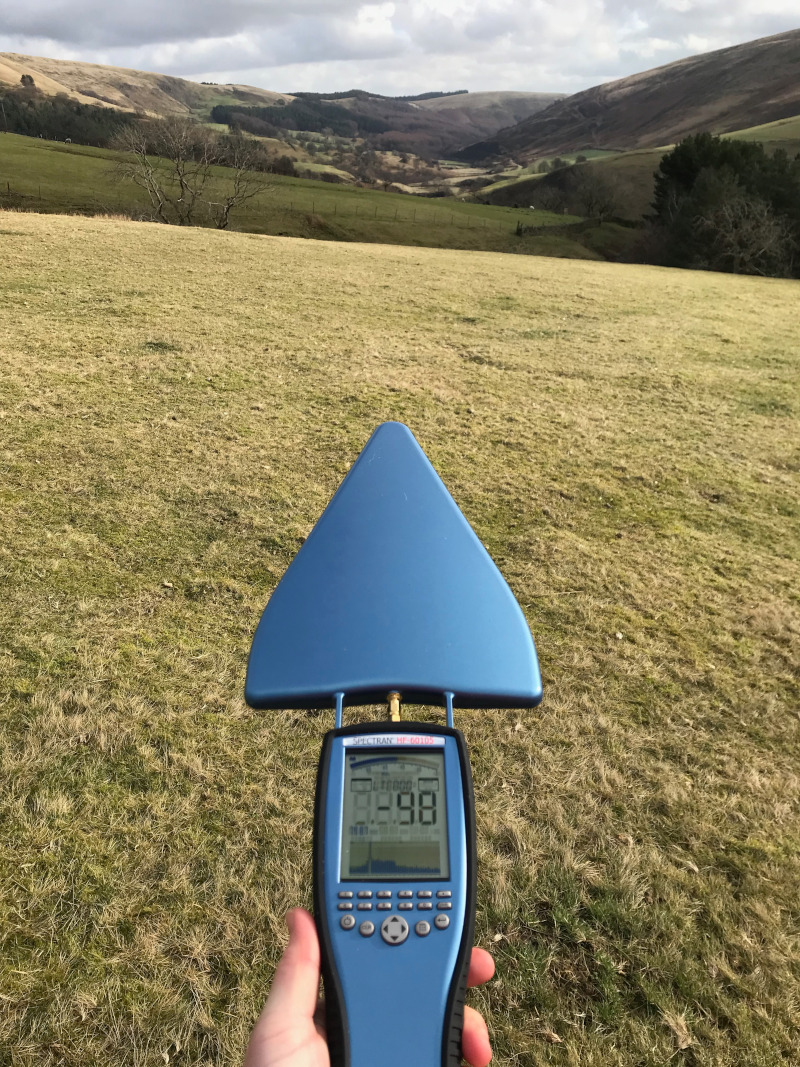
The colour schema can be whatever you like but if you want to align with the ‘S’ meter scale, popular with HF, where a barely workable signal is S1 and the best is S9 (-73dBm) use a max value of -73dBm with 6dB bands for S9 to S1.

Accuracy verification

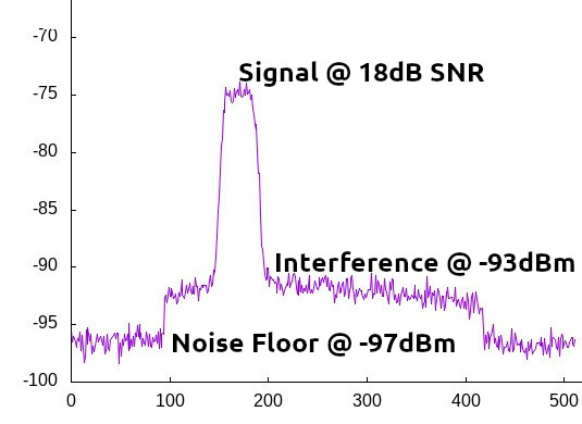
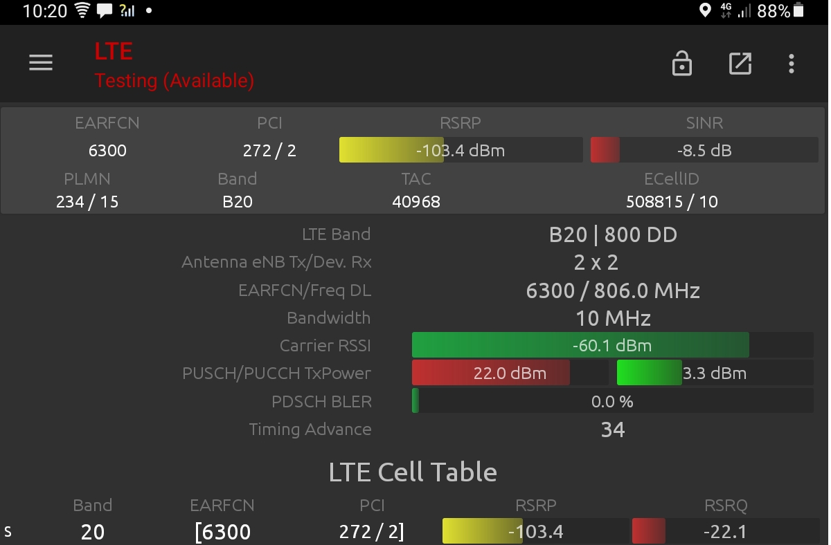
We have calibrated our NVIS model to align within 10dB of measurements taken from a 2012 research paper by Marcus Walden using a 5MHz NATO frequency in the UK. From this paper we selected one of the longer links at 210km where we used the median measurement value which for August 2009 was lower during the day than VOACAP, a popular open source application for HF forecasting. The median dBW measurement at noon was -120dBW (-90dBm).

Noting that the RMS error between the VOACAP predictions and the measured values was concluded to be 7 to 12dB at 12 noon (Ref table 7 on page 8), and more at night, we have tuned our model so an “optimistic” prediction is 3dB from the noon measurement. The context and reliability options provide sufficient control to allow predictions to align with current and local ionospheric conditions.

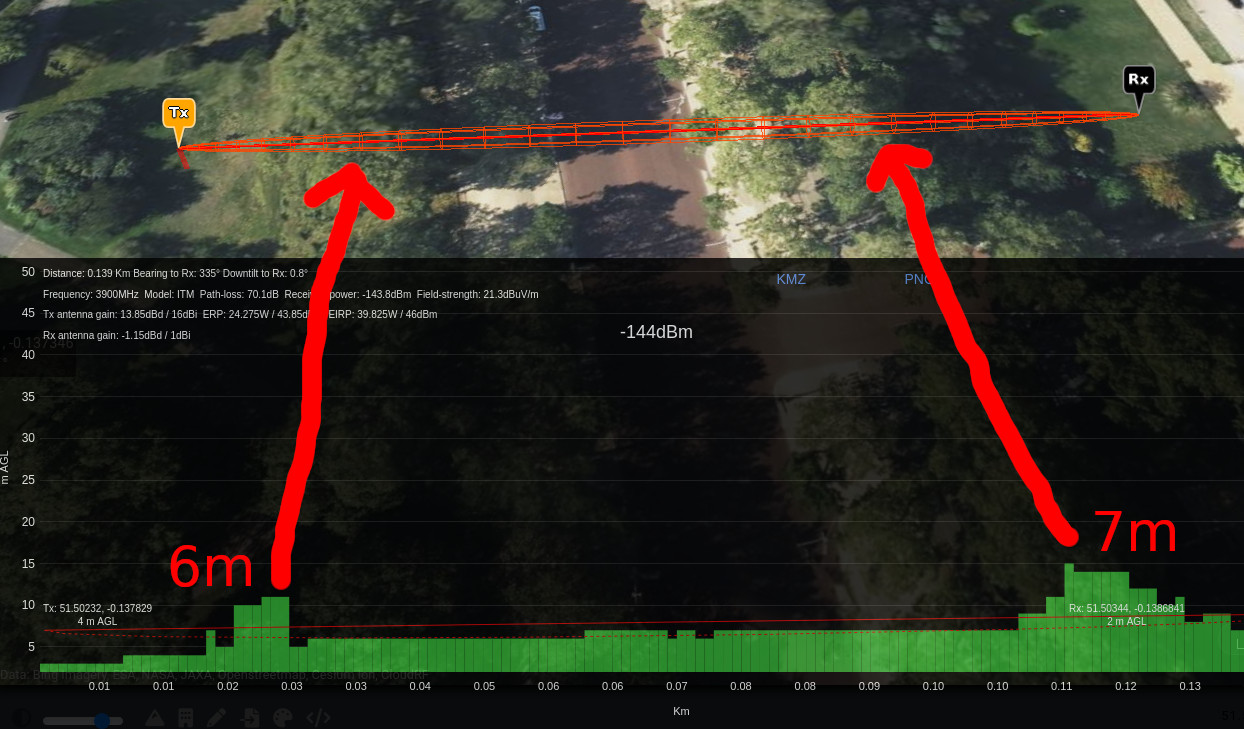
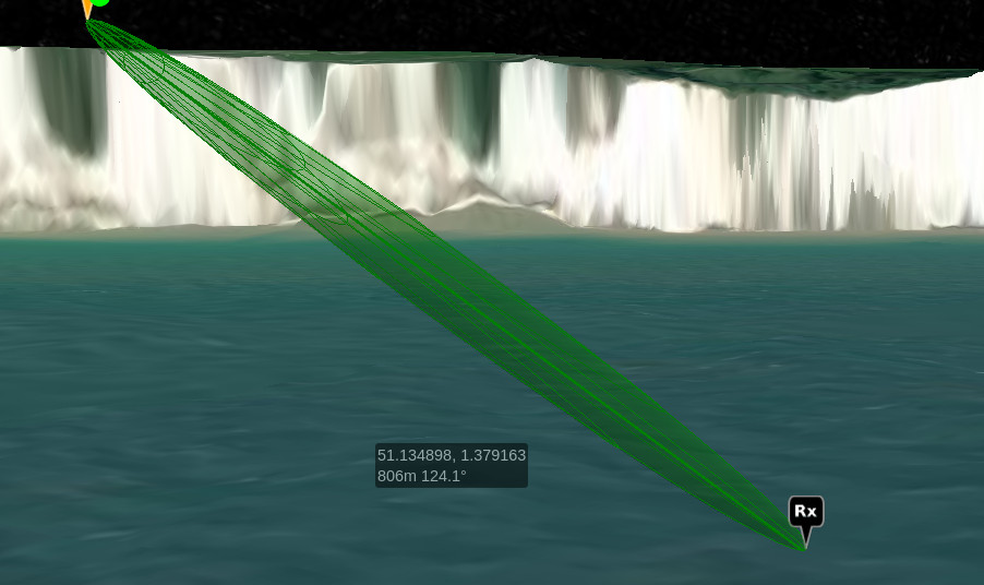
The screenshot below shows both the path and the area coverage aligning with a 1dB calibration schema. The link has over 900m of curvature height gain which explains why a flat region of England appears as a mountain!

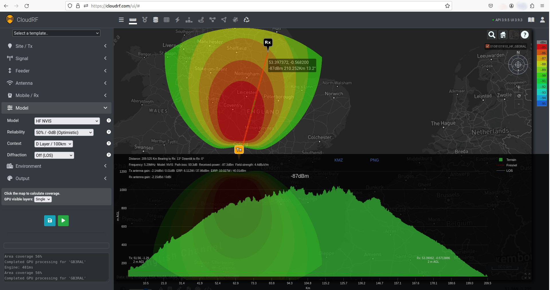
Ionospheric modelling is less predictable than terrestrial modelling due to unpredictable solar radiation. Predictions generated with this model are useful for training, situational awareness and antenna alignment but cannot provide an accuracy greater than 10dB, assuming the inputs are correct.

Look forward: Space weather and long range HF

HF forecasting tools use lookup tables to set refractivity during both seasons and times of day. Using quality, and current data, improves accuracy but like weather forecasting it cannot offer accurate predictions without live data, in this case space weather which has seen a lot of renewed research recently. Our implementation does not use forecasting data presently so users should not be using it to pick their frequencies, but it will help visualise the coverage and align antennas – which at 500km is important.

For the next phase of HF, long range skywave, we will use a space weather feed to offer high resolution HF predictions. Long range HF uses multiple hops at lower angles so the space weather and time of day must be considered along the route which may be thousands of kilometers….

Posted on 2023-05-082024-04-16

Critical Coronation private 5G network planned with CloudRF

On Saturday 6th May the worlds media descended on London for the Coronation of King Charles, an event last planned before many people had television.

As the national broadcaster, the BBC managed the coverage and worked with Neutral Wireless to deploy an innovative private 5G network, with dedicated spectrum, along the procession route for exclusive use by the media and special cameras with 5G modems.

Using the CloudRF API with UK LiDAR data the team created accurate urban line of sight models for their N77 base stations along the tree lined route. Their model used RSRP units and a custom colour schema to map the 4GHz downlink coverage and key handover regions to ensure smooth subscriber transitions for the dynamic event.

Antenna patterns

The area to be covered is a linear tree lined boulevard known as “The Mall” which leads to one of the most iconic buildings in the country, Buckingham palace. For this task, high performance Alpha Wireless directional panels were employed above the crowds at only 4m, much lower than a conventional city cellular network where a mast will be on rooftops. The combination of low height and a 4GHz frequency limits the effective range so the direction of the antennas needed to be carefully optimised to provide maximum coverage for broadcasters, strategically positioned along the route for line of sight.

How do you model a parade of horses?

Given the low height of the masts and the significant number of tall horses on parade this presents a challenge to critical line of sight which a LiDAR vendor cannot help with. The same problem applies to temporary structures such as the grandstand erected outside the Palace.

For a challenge such as this we can use custom clutter to simulate a parade of horses at a uniform distribution with a nominal density value. A “brick” clutter type can be customised to 2m height and 0.4dB/m attenuation to simulate loss through the parade to show the low and high risk locations for maintaining a link through the parade.

Our current 2D engine regards all obstacles as extending to the ground so a clutter model for a horse will be conservative since in reality a horse has a substantial gap between its legs sufficient for some RF to travel between it and reflect, and diffuse, off the rough ground to reach a camera beyond it. We’re already working on 3D 😉

In the screenshot below, the formation nearest the mast present no challenge, the formation in the middle show attenuation throughout them making a link difficult potentially depending upon siting of the receiver and the distant formation is blocking the, already attenuated, signal.

Trees

The parade was held in May when the trees along the Mall are coming into leaf presenting a moderate obstacle to the 4GHz frequencies. The temporary masts were therefore erected forward of the trees for optimal coverage but still technically under the canopy which makes planning challenging with a 2D engine since these trees can exist as spikes in the LiDAR profile. To avoid accidentally siting a mast atop a tree/spike in the model the path profile tool can be used to inspect the path profile, to identify where there are tall trees in the underlying surface model. Using the UK Environment Agency LiDAR from 2019, the nearest trees on the Mall are lightly represented in LiDAR with a 6m to 8m average canopy compared to their significant neighbours one row back and beyond in St James Park.

The result

The high resolution coverage map was integrated with official event mapping, printed, and displayed in the event broadcasting operations room as a reference. You can also see it on the BBC.

Despite the challenges expected from such congested spectrum, dynamic obstructions and the unexpected surprise of unscheduled electronic counter measures they were able to deliver accurate coverage, on time and within budget to broadcast a historic event in high definition, in real time.

CloudRF referenced in award winning technical paper

The BBC research and development team published an award winning paper at the 2023 International Broadcasting Convention about the event titled 5G Standalone Non-Public Networks: Modernising wireless production.

In this paper, the 4GHz coverage accuracy was validated using ground truth data. This quote about CloudRF’s accuracy stands out:

The agreement between the predictions and on-the-ground measurements is excellent
BBC Research and Development

You can download the paper at the BBC here.

Posted on 2022-10-242022-10-26

Bandwidth and noise

As communications systems have grown in capacity, they have expanded in physical bandwidth in an increasingly congested RF spectrum.

Effective digital communications planning requires more than knowledge of antennas and propagation fundamentals. It now needs an intimate understanding of bandwidth and noise to co-exist and communicate efficiently.

Unfortunately, this key aspect of modern RF systems is often taught badly, or in some cases not at all, leading to often unwelcome surprises for equipment operators in the field. As a technology and market agnostic platform we’ve observed poor bandwidth knowledge in many markets, but notably MANET and 5G, both of which are accelerating the deployment of wideband systems, often with little to no planning beyond a topographic map study.

Both radio markets are evolving from narrower channel technologies, which in the case of MANET and the VHF Combat-Net-Radio (CNR) it replaces was measured in KHz so they need to update their theory training content and associated software to convey these potentially complex topics to novice students in a digestible manner.

Increasing bandwidth increases noise, which reduces coverage

Teaching noise

As bandwidth increases, so does channel noise. This simple concept might seem easy to remember for a student but without visual aides, and since the demise of analog systems; audible aides, it is hard to demonstrate in practice.

A good teacher may show visual aides like noise charts, FFTs, spectograms and a bad one may show some Johnson-Nyquist formulas buried within an all-day powerpoint which is not helpful except for getting paid.

FFT showing a narrow signal and wideband interference

A student can tick the right box on their exam(s) but spend their career wasting bandwidth and struggling to establish communications because they believe that big is better – it isn’t, or worse still, that bandwidth has no effect on the coverage since that’s a function of transmitted power and/or height. Having an intimate understanding of the interplay between bandwidth, receiver sensitivity and thermal noise will make spectrum users more efficient, effective and considerate.

Bandwidth MHz	Thermal noise (dBm)
0.1	-124
1	-114
2	-111
4	-108
8	-105
16	-102
32	-99
64	-96

Bandwidth thermal noise table based on a temperature of 21C

Which waveform is best?

Comparing digital radios is complicated due to the myriad of features, waveforms and software.

Given a particular waveform it will have characteristics such as a minimum Signal-to-Noise Ratio (SNR) value which it requires to achieve a symbol rate necessary to deliver a fast data link for example. This dB value must sit proud of the noise floor so if the noise floor is high at -90dBm, coverage will be reduced and conversely, by taking it to somewhere quiet eg. -110dBm, the coverage will improve by 20 decibels – a huge difference.

To compare waveforms precisely, the same noise floor should be simulated, initially, with fixed values to eliminate random error in field testing. The sensitivity values will be somewhere between 3 and 20dB depending on what the waveform and target Bit-Error-Rate (BER) is.

Bit Error Rate (BER) describes the ratio of errors in a data stream. An ok value is 10^-3 or 1 bad bit in a 1000 or 0.1%. This increases with noise until a signal is unrecoverable. For more on BER see an older blog here.

For ground radios designed for noisy environments, a BER of 10^-2 (1 error in 100 or 1%) is used here for extracting our planning thresholds from a chart of SNR curves. For an airborne system without obstacles this could be higher, for example 10^-5.

Signal to Noise Ratio for different modulation schemas against error rates.

A narrow waveform eg. QPSK gives better coverage and works better in noisy conditions. This is the fallback telemetry mode used in many data radios.

A wide waveform eg. QAM64 is capable of better throughput and delivering high bandwidth streams such as HD video.

The best radio is one which can use different waveforms to satisfy both coverage and capacity.

Modelling bandwidth: A tutorial

Modelling RF Bandwidth and noise

Quick reference guide

A quick reference guide for using bandwidth and noise is available here. For other guides see here.

221025_SNR_quick-guide Download

Conclusion

Bandwidth and noise is essential knowledge for anyone deploying wideband systems or comparing waveforms.

RF theory training can be enhanced (and needs to be) with visual tooling to let students quickly observe the impact of different inputs in a controlled environment with templates to minimise user error.

For information on how SOOTHSAYER can help with signals training see here.

Posted on 2022-02-202022-02-20

Improving LTE modelling with field test data

We took a field trip to model LTE (4G) coverage in order to collect data we can use to develop calibration utilities and improve modelling as modelling is only as accurate as your inputs.

We focused on a single remote cell in the Peak District national park identified through cellmapper.net. We expected to find one cell only but were surprised to be serviced by several distant LTE cells, not evident in the crowd sourced app and equally significant, we established limited or no coverage in an area where a national map suggested coverage was available.

Key findings

Data revealed the crowd-sourced coverage app was conservative in rural areas
Data revealed the operator’s network map was optimistic in rural areas
Modelling was matched with 2.5dB RMSE for a cell 12km away
Modelling was on average accurate to 5.5 dB RMSE
Improvements to modelling have been identified

Equipment and process

We used a rooted Samsung Galaxy Tab with an integrated Qualcomm X11 LTE modem, running both Network Signal Guru (NSG) and Cellmapper. NSG requires root access to lock to a cell which was necessary to prevent our survey tablet from hopping around not only protocols (2G,3G) but neighbouring cells.

Cellmapper is a crowd-sourcing app which writes signal strength readings to a CSV file, convenient for our analysis. Before embarking we planned a route around a remote cell on the edge of available coverage maps.

Both apps record various LTE power levels such as Received Power Received Signal (RSRP), Received Power Received Quality (RSRQ) and Received Signal Strength Indicator (RSSI). For this test we use RSSI which is typically a stronger value than the others as it is the measured carrier, irrespective of bandwidth.

Receiver measurement calibration

Radio receivers are subject to measurement error, typically in the range of 0.5 to 3.0dB for very expensive and consumer grade equipment respectively. As we were using a consumer grade Snapdragon 662 SoC with an X11 LTE modem, we needed to find out it’s measurement error. The Qualcomm datasheets we could find didn’t list this value so we used empirical measurements to establish it.

During our survey we paused at a site 3km from a tower with line of sight where we recorded continuous power readings with the tablet static on the ground for about 15 minutes. Consistency is essential for calibration. We have analysed these readings to establish a standard deviation in readings of 3.1dB for the X11 LTE modem, which puts it at the consumer end of the spectrum for survey device accuracy, in accordance with its price.

We use the error of 3.1dB in our analysis by subtracting it from the Root Mean Square Error (RMSE).

python3 receiver_calibration.py receiver_calibration_3km_LOS.csv 
[-71.0, -71.0, -67.0, -71.0, -67.0, -69.0, -69.0, -69.0, -71.0, -77.0, -67.0, -71.0, -73.0, -71.0, -71.0, -71.0, -75.0, -69.0, -73.0, -69.0, -75.0, -69.0, -71.0, -79.0, -73.0, -65.0, -73.0, -71.0, -71.0, -75.0, -71.0, -73.0, -77.0, -75.0, -69.0, -75.0, -75.0, -73.0, -77.0, -73.0, -71.0, -75.0, -73.0, -79.0, -75.0, -71.0, -71.0, -75.0, -67.0, -73.0, -73.0]
Mean: -72.1dB
Error: 3.1dB

The survey

Setting off uphill from Derwent Dam car park with Sheffield’s man-of-the-mountain, Chris, we approached our target cell located on the hillside below us.

As we neared 500m we used NSG to lock onto a strong LTE signal which we believed was the target (CID 130256660, PCI 270), based on proximity and strength (-60dBm RSSI). It was in fact a tower on a distant hill 12 km to the south with line of sight, CID 131413770. Surprise number 1.

Field testing in the Peak District

At the top of the hill we could see the target tower’s directional panels which confirmed it was configured to serve the A57 “Snake pass” road below. One panel was oriented north-west towards Manchester (CID 130256660) and the other south-east towards Sheffield (CID 130256650). Based on the dimensions of the panels we estimated their beamwidth as at least 120 degrees and gain of at least 10dBi.

As we passed the eNodeB along the hill top we were conscious of a number of cell neighbours and performed a targeted re-selection where we ended up briefly attached via the antennas back-scatter of *6650, made possible by our proximity. This didn’t last for long before we re-selected to a strong signal (PCI 337) which we were convinced was CID *6660. It wasn’t. Surprise number 2.

Surveying LTE cells with Network Signal Guru

We later found out this was also a distant cell with line of sight near Hope, 7km due south of us!

Marching on happily with a great signal, we started a gentle descent until we lost the horizon behind us. At this point the neighbours we observed disappeared and our serving cell (in Hope) became very weak as we entered the signal’s (diffracted) beyond-line-of-sight (BLOS) shadow. As predicted in the video based on the surrounding high plateau we could see, we lost the signal as we continued to head north toward Alport Castles, a local feature. We descended into the valley below without a signal (despite a national map suggesting otherwise) and continued the next 3.5km without any coverage at all 🙁

Losing all cells on a high plateau

As we exited the remote valley, heading towards the A57 road, we reacquired a signal and finally locked onto our target, *6660, with an excellent signal and line of sight (Credit to Chris for spotting the tower in the trees at 2.7km!). As observed, the directional pattern was focused on the road and we were in the main beam.

Acquisition of the target cell

A quick map study and we elected to march west until we lost the signal. This event occurred after only 1.5km thankfully as we hand railed the road over undulating terrain. We followed the same route back to the acquisition point which doubled our measurements for this section.

Confirming the direction of the powerful 10MHz LTE800 bearer with a portable spectrum analyzer with a bad LCD.

From the A57, in the main lobe, we climbed the hill to the south east and headed back toward the target cell. Knowing it had a directional pattern, we anticipated signal strength decreasing as we exited the main lobe which we confirmed as we drew parallel with the cell, eventually circumnavigating it to the south.

As we exited the beam of *6660 and entered the influence *6650 we re-selected for the final phase of our journey which would take us into a steep ravine and then up the hill, right past the cell.

A sweaty climb up a steep hill behind the cell, saw signal strength and field testing enthusiasm collapse which was fixed with some fizzy snakes. We lost the cell for good only 500m behind it due to the convex hill and directional pattern.

Moral of the story is, in RF, proximity to an access point is no guarantee of service!

Serving cells

Cell ID	PCI	Location	Technology	Frequency	Comments
130256650	272	Hagg Farm (South East)	LTE Band 20 10MHz	806MHz DL	~15m AGL
130256660	270	Hagg Farm (North west)	LTE Band 20 10MHz	806MHz DL	~15m AGL
131377930	337	Hope Quarry	LTE Band 20 10MHz	806MHz DL	~15m AGL
131413770	441	Little Hucklow	LTE Band 20 10MHz	806MHz DL	~20m AGL

Table of serving cells featured in our data

The cells all have a downlink and an uplink frequency. As these four cells share the same downlink they are separated in time using a multiplexing schema and the Physical Cell Identifier (PCI) code. If we only took out a spectrum analyser we’d never know which cell we are looking at otherwise.

Data analysis

We chose to model after field testing. We could have done it before but it would have ruined all the surprises that came up during analysis like the serving cell 13km away!

We extracted the CSV data (1034 rows) from the survey tablet which for cell mapper was located at /storage/emulated/0/Android/data/cellmapper.net.cellmapper/files/.

We sorted it by cell and created clean CSV files for each cell with only the location and RSSI.

Gap analysis

Formatted CSV data. group = CID, id = RSSI

We used our new “coverage check” CSV import tool. This tool allow the import of customer locations which can be tested against visible coverage layers to report a correlation.

This is a binary yes/no comparison with a summary report eg. “87% coverage” which is handy for comparing options.

It cannot automatically calibrate field test measurements but is useful for gap analysis as a “first pass” toward calibration.

This tool is handy for manually aligning the modelling until it matches visually but is too simplistic for calibration.

Coverage check tool showing an 87% correlation. The deadspot is where modelling was conservative.

Fine tuning inputs

Our confidence level for the inputs started around 50%, based on known frequencies, heights and power levels for the UK network. For the first cell, we used a combination of known, observed and assumed values.

You can be forgiven for thinking why not do field testing with known transmission parameters but even then you must calibrate as old batteries, weathered connectors and battered antennas will all impact a transmitters actual effective radiated power (ERP).

As we working LTE800 we used the ITM model, designed for this UHF band when it was conceived for TV broadcasting. This general purpose model has built in diffraction and also has a reliability variable which we can use for fine tuning.

Known values: frequency, location, approximate height, approximate azimuth
Estimated values: Antenna azimuth, beamwidth, gain, RF power, exact height

Once we had a coverage plot using some sensible power values and the coverage-check tool reported a correlation > 90% we rendered it using the Greyscale GIS colour schema and download a GeoTIFF raster. This contains fine grain signal values to 1 dB resolution.

Calibration process

We suggest this workflow for the calibration process.

We also have an API capable of returning data in open vector and raster formats including SHP and GeoTIFF so there are other ways to do this...

Gap analysis with the coverage check tool in the web interface and approximate/rough inputs
Power balancing with the path profile tool for selected points only (Recommend a LOS link at long range)
Gap analysis with the coverage check tool in the web interface and power balanced inputs
Regenerate the layer with the GIS schema and export for precision offline calibration
Make minor (1-2dB) adjustments to either the loss or gain values for LOS links, and/or clutter profiles for BLOS until the calibration script reports an RMSE value < 10.

Offline calibration

Using a Python script and the rasterio library we were able to query each row from the CSV data against the GeoTIFF raster instantly, negating the need for many recursive API calls.

The offline method is more efficient when working with large point-to-multipoint layers and spreadsheets than calling the API directly. It computes a mean error which can be positive or negative and a more useful root mean square error (RMSE) which is always positive. A lower figure is better with 0dB being ideal (and also impossible).

The API method is still valid for testing select points or calibrating dynamically.

python3 Offline_Calibration.py 131413770.csv 131413770.tiff 
...
Lat: 53.402250 Lon -1.760703 Measured: -65.0dBm Modelled: -68.0dBm Error: 3.0dB Mean error: 0.5dB
Lat: 53.402252 Lon -1.760699 Measured: -59.0dBm Modelled: -68.0dBm Error: 9.0dB Mean error: 0.6dB
Lat: 53.402253 Lon -1.760699 Measured: -61.0dBm Modelled: -68.0dBm Error: 7.0dB Mean error: 0.7dB
Lat: 53.402252 Lon -1.760698 Measured: -63.0dBm Modelled: -68.0dBm Error: 5.0dB Mean error: 0.8dB

Model error is mean 0.8dB, pure RMSE 5.6dB based upon 84 measurements
Receiver measurement error: 3.1dB
RMSE adjusted for receiver error: 2.5dB
The modelling inputs are excellent.


RMSE	Description	Comment
0 to 3	Excellent	Calibrated!
3 to 6	Very good	Inputs are very close. Fine tuning needed.
6 to 9	Good	Inputs are good but more tuning needed
9 to 12	OK	Inputs are OK but not tuned
> 12	Bad	Inputs are bad. Check basics eg. Height, Frequency, Power

Suggested interpretation of calibration scores. Requirements will vary by scenario.

The results

We achieved results better than expected. We were aiming for under 6dB RMSE and achieved 3dB, at 7km range, which is excellent, and coincidentally as accurate as the measurement accuracy of our survey device.

Manual calibration can be time consuming, and collecting good data definitely is. We felt we could have improved the scores further with more data, like the antenna data sheets for starters, but were happy with our 3dB.

The good

The best results came from the distant cells where LOS was achieved. This makes sense as without obstacles to complicate things the path loss decays at a predictable rate, based on wavelength, which can be plotted as a clean curve. Once we had this power balanced using the path profile tool and manual adjustments, it produced a great match with the data due to the open nature of the high plateau.

Calibrated modelling for a cell 7km away with line of sight

The ugly

The other cells, like our target at Hagg Farm (South east), served a more complex piece of ground in the valley which had steep ravines and tall trees. As expected we didn’t fair as well here and achieved 10dB RMSE. Analysis of where we lost accuracy can be summarised as follows:

Trees. We found 2m LiDAR to be too conservative here as this contains the tree canopy. We tried smoother DSM with clutter profiles which gave a better result but didn’t go as far as adjusting our clutter profile. This is a future trees blog!
Proximity. Counter-intuitively, being closer to the cell is not better for measurements and calibration than being further away. This is due both to the way path loss decays on a curve and the highly directional panels cells use. Small differences near a cell produce large differences in data, compared with very small differences up on the plateau with the distant LOS cells. We can model directional panels but are guessing what the *actual* beamwidths are.

Cell	Points	Mean	RMSE
130256650	164	-0.7	9.8
130256660	460	0.9	6.9
131377930	127	-1.6	3.0
131413770	84	0.8	2.5
TOTAL	835	-0.15	5.5

Table of scores for the calibration of the four measured cells

Look forward

The so what of all this is we have proven the software is capable of high accuracy, given the right input, and we have identified areas to improve it further.

We will be adjusting our LiDAR to soften it in areas where this is available to fully exploit recent developments with our custom clutter profiles.
We will be integrating recent developments with offline calibration into our user interface to make this manual process smoother, simpler and faster.
We will work on automating calibration. Some might call this machine learning blah but it’s just software.

Expect another field testing blog all about……trees.

Consolidated and calibrated LTE coverage for the valley, served by four cells

Scripts and data

You can download our field test data and Python scripts here as well as Google Earth KMZs showing the route,cells and measurements.

LTE_FIELD_TEST Download

Posted on 2021-09-28

Modelling microwave links over the horizon

In this study we look at modelling long range microwave links and the key parameters which help get the best out of mobile microwave terminals. When sited properly, a low power microwave terminal can communicate over 100km. When sited badly the same terminal can fail to communicate 5km…

A brief history of microwave

Commercial terrestrial microwave links spread in the 1950s during post-war radio innovation and are used today as backhaul in many key public and commercial networks. A microwave station typically consists of a large tower on high ground with round parabolic dishes communicating in UHF (300MHz) bands and above. As Wi-Fi spread after the millennium, outdoor fixed wireless access (FWA) terminals for long-range (>2km) consumer wireless links became increasingly popular, especially around ISM bands, but only recently have portable tracking terminals like the AVwatch MTS become available, intended for mobile ground to air use at distances exceeding 150km.

The theory

A microwave link is designed to be high capacity and focused in order to carry a large amount of information from one point to another. For this reason they need a short wavelength so are found in UHF and SHF bands above 300MHz.

The signal has a fresnel zone around it which is sensitive to obstructions. Achieving a line-of-sight link is not a guarantee of a good connection if the fresnel zone is obstructed by trees or buildings. The size of this zone is inverse to the frequency so a higher frequency has a smaller zone, akin to a laser beam, compared with a lower frequency which has a larger zone and so requires to be higher above the earth to clear it.

Radio horizon

The maximum distance a microwave link can go over the earth has little to do with RF power and much more to do with the dish heights and the horizon which limits how far a (short wavelength) signal can go. Whilst refraction can extend a link beyond the horizon, it is variable like the weather so impractical to model accurately and in a timely fashion. A simple formula to calculate the radio horizon is 4.12 x sq(height) where height is the combined transmitter and receiver altitudes. This formula produces a table of horizons which show that an improvement in height of several meters translates to a range improvement of several kilometers due to the earth’s curvature.

Transmitter height m	Receiver height m	Radio horizon km
1	1	6
1	10	14
1	50	29
1	100	41
1	200	58
1	400	82
1	800	116
1	1600	164

Parabolic antennas

As signal attenuation is substantial at these frequencies they require a highly directional antenna to improve forward gain and cancel noise from other angles. The larger the dish size the greater the gain and the smaller the beam.

A microwave dish antenna is easily recognised as a polar plot by it’s prominent main lobe, symmetrical side lobes and minimal back scatter. It has a very high front-to-back ratio which describes the ratio of forward power to rear in the order of +50dB. Due to it’s high directional gain it only needs to be driven with a modest amount of RF power to generate an effective radiated power of several hundred watts.

Using and creating a directional pattern

In CloudRF you can choose from thousands of crowd sourced patterns, upload your own in TIA/EIA-804-B / NSMA standards or create your own using a few parameters.

To select a template, open the Antennas menu in the web interface and click the database icon. This will open a search form. Search by manufacturer, eg. Cambium, or model. When you find a pattern you want click the green plus symbol to add it to your favourites list. You can now proceed to set the azimuth and tilt as if you were affixing it to a pole.

If the pattern does not exist, you can choose to use a “custom pattern” and define the horizontal and vertical beamwidths in degrees as well as the gain and front-to-back ratios in decibels to generate polar plots. These can be downloaded as a legacy .ant text file which you can upload in the service as a private pattern. A custom pattern is quick to self-generate but lacks side lobes and the full accuracy of a detailed pattern from a manufacturer.

An over the horizon link

For this demo, we’re simulating a link from the cliffs of Dover in England across the English Channel to Calais, France, a distance of 40km across the sea with no obstructions. The 18dBi terminal is 1m off the ground and is using only 3 Watts / 34.7dBm power for a total effective radiated power of 189W / 52.8dBm. A receiver threshold of -100dBm was used. This is too low for high speed waveforms but would be ok for a telemetry fallback waveform like QPSK.

A bad link

With a ground receiver on top of the cliff, the link just reaches Calais. It is obstructed on the radio horizon at ~25km, a full 10km before the coastline but the height advantage of the cliff makes line of sight just possible to some parts of the town. Despite just achieving line of sight, this link would still be unsuitable due to the majority of the fresnel zone being obstructed.

A good link

With the same cliff top terminal and RF parameters, the distant receiver is swapped for a drone 300m above the ground. The increase in height extends the link from ~25km to 75km, deep into France with good LOS.

An ugly link

This time the same terminal which just achieved 75km was misused down on the beach to communicate with a small boat in the channel. It’s effective range was less than 6km due to the radio horizon. As you can see from the normalised path profile chart below, the curvature impact is substantial when the stations are on the earth!

Thresholds and modulation

The simplest way to limit the modelling is with received power measured in decibel milliwatts. In this common scale, -100dBm is a sensible threshold for most digital systems. For planning purposes, a 10dB fade margin should be added for a -90dBm threshold. The actual thresholds needed will vary by systems and waveforms. Many commercial microwave links operate very high symbol rate modulation schemas which need received power above -70dBm to function.

You can also use Bit-Error-Rate (BER) as a threshold. This unit is used in conjunction with the noise floor and the desired signal-to-noise ratio (SNR) to derive a threshold. A modulation schema like QAM64 requires a relatively high 15dB SNR compared with 5dB for QPSK which can function on weak links. These thresholds are not absolute which is why we set the desired error rate. Errors are inevitable and the relationship between the BER and SNR is best visualised as curves. If you know you want QPSK for example but are not sure what error rate to use, use a mid level error rate such as 10-3 (One bad bit for every 1000 bits) which will give you a 7dB SNR. If the local noise floor is -120dBm your equivalent receiver threshold is a pretty low -113dBm.

Conclusion

Forget RF power, height is everything in creating a successful microwave link. This might mean moving a terminal several kilometers away from the distant station in order to gain a few meters in height but the benefit will be many more kilometers in range.

Posted on 2018-04-302021-05-22

Adding antenna patterns

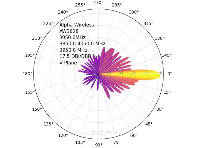
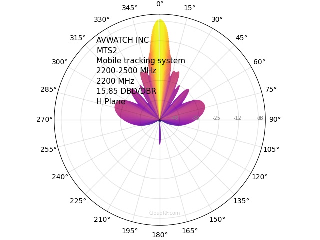
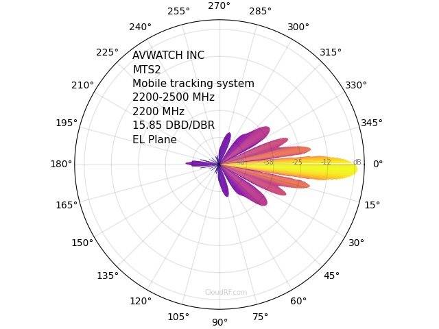
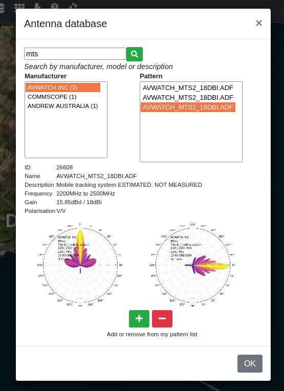
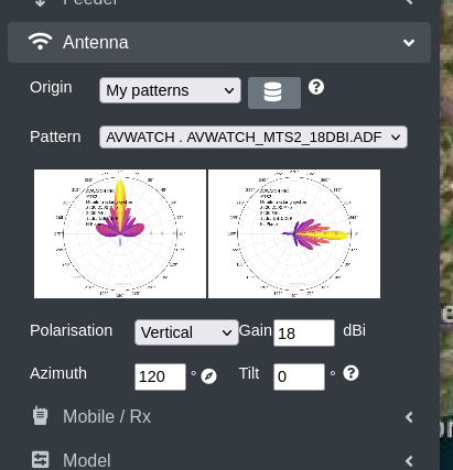
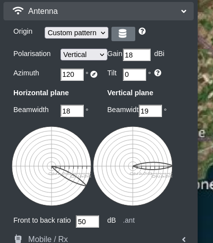
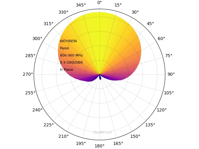
You can use ADF / NASM (TIA/EIA-804-B standard) and ANT patterns in CloudRF. These basic text formats are open and easily edited and will display a patterns azimuth (Horizonal plane) and elevation (Vertical plane), typically as 360 rows of data each. ADF pattern data is generally in dBd and ANT is a normalised range with 0 as peak power. ADF is the primary pattern format and all ADF patterns are public (accessible to all users). ANT is the secondary format and is private (accessible only to the uploader).

Feature	ADF	ANT
Access	PUBLIC	PRIVATE
Azimuth	360 rows	360 rows
Elevation	360 rows	360 rows
Metadata	Name, OEM, Description	Name
Frequency	Defined range ONLY	Any
Gain	Defined gain only	Any
Polarisation	Defined only	Either
Tilt	At time of use	At time of use
Rotation	At time of use	At time of use

In summary: ANT gives greater freedom but is risky. ADF ensures correct inputs.

Finding a pattern

There are thousands of antennas from over 21 OEMs. To find the ones you need/want, use the database search feature by firstly typing in your frequency eg. 100 (MHz) and clicking search to filter the results and finally typing into the search box eg. Dipole to find the closest match. You can sort results by any of the columns by clicking it. Next click the hear to add it to your favourites. It will then become available in the interfaces in your selection. This is unrelated to the API which will let you use any pattern if you know the ID number (in the table). If you can’t find your pattern you can source it from the manufacturer in ADF / NASM format.

Kathrein Antenna Patterns

http://www.rfiwireless.com.au/base-antennas/patterns.html#.Wud18nUrL0o

Antenna Pattern Files

Upload a public ADF pattern

Method 1: Login to the web interface then click the antenna database icon within the ‘Antenna’ input menu. Method 2: Login to the web interface then visit https://cloudrf.com/antennas Click the ‘Add public .ADF pattern’ link to access the form and then upload your ADF pattern. Any formatting errors will cause a failure which you will be notified of. Ensure your ADF data contains valid metadata in the header eg. gain, name, description. Any data deemed erroneous or inappropriate will be removed from the system without warning.

Upload a private ANT pattern

Method 1: Login to the web interface then click the ‘My Patterns’ button in the Antennas menu Method 2: Login to the website then click ‘Antenna patterns’ on the homepage Click the ‘Add private .ANT pattern’ link to access the form and then upload your ANT pattern. Any formatting errors will cause a failure which you will be notified of. Ensure your ANT data contains 720 rows of data (Azimuth followed by Elevation). Do NOT apply rotation or tilt as this is done dynamically at the time of use. Any data deemed rotated, tilted, erroneous or inappropriate will be removed from the system without warning.

Using patterns

Your uploaded pattern won’t appear in the web interface immediately. You must reload the list with the reload button next to it, especially if you’ve just updated your favourites.

Old ANT patterns

Don’t worry they didn’t get deleted. You can find a list of them here.