Interference is one of the single biggest issues in radio which limits the potential of a system or network.
There are different types of interference but the problem of interference visualisation is common to all. With simulation software you can model your system, and an interfering system, but understanding the interplay where the coverage of the two overlap is crucial. Like many radio engineering concepts it’s a complex topic so making it simple requires abstraction which our API provides.
Up until now we offered a basic interference capability, capable only of colour promotion. It was unable to consider signal parameters or to show the level of interference.
Enhanced Interference API
The upgraded interference API considers the signal parameters frequency, bandwidth and power. It accepts two arrays of sites, one for the “signal” network and another for the “noise” network so you can compare two sites or scale the concept for two networks.
Frequency is obvious as two local signals on the same wavelength will interfere. This technology agnostic API considers the signal as a constant carrier. This means it does not consider features of the waveform since modern technologies, like 802.11, employ back-off mechanisms in the PHY to manage collisions whereby a transmission will pause momentarily if it detects noise.
Bandwidth is important as even if the signals are on different channels, their bandwidth may overlap. In 802.11, adjacent channels overlap by design when using wide (20MHz) signals but the amount is small enough that the spread spectrum signal can overcome it in error recovery mechanisms. As a result, many signals can operate in a dense slice of spectrum.
Power is harder to plan for in spectrum planning where the focus is normally on frequency management and is the source of most interference reports. Even if two signals are on different channels, with non-overlapping bandwidth, they can still interfere if one of them is sufficiently powerful. This is because a signal produces frequency harmonics at multiples of itself and power in the spectrum appears as a Gaussian function which looks like a bell curve. A powerful signal will bleed power into the spectrum adjacent to it and if a receiver does not have an adequate filter, it will receive this power even if it’s on an adjacent channel!
Presenting interference

We use decibels (dB) as the measurement unit to describe interference along with a special purpose colour key called JS (Jam to Signal). The J/S ratio, as the name implies, shows the interference (Jammer) power over the signal power. A bad JS ratio implying strong interference would be greater than 0 eg. 12dB and a good ratio would be negative eg. -12dB.
The level at which this interference presents a problem to a given waveform varies. Some waveforms are designed to operate within noise such as LoRa and others like WiFi fail gradually with noise: When people say “the WiFi is slow” yet they have a strong signal, the problem is interference which causes sampling errors, and reduces data bandwidth.
Using -3dB as a interference limit in planning is recommended. This is green on our colour key.
Anything higher than this and there will be reduced performance / speeds. An interference ratio higher than 0dB will likely stop you communicating altogether if your signal requires a positive SNR ratio – as most do. For reference, high capacity data waveforms require 20dB SNR and commercial telemetry requires less at 3dB SNR.
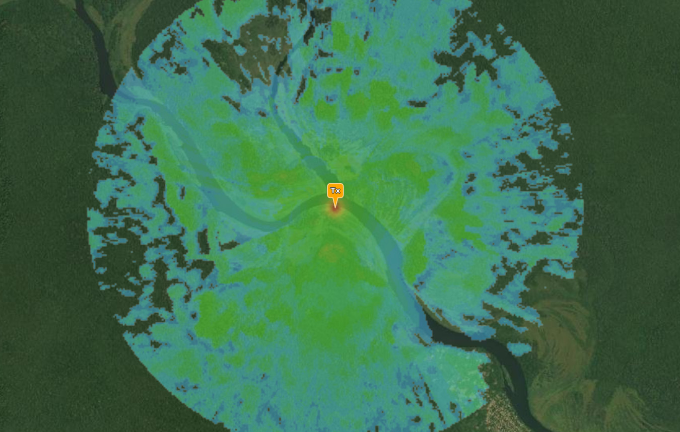
Demo: Signal jammer (Frequency)
This high resolution frequency demo shows the impact of a 10W signal jammer against a high powered urban rooftop cell tower radiating ten times more power at 100W EIRP.
Despite being near to the strong, and elevated, cell, the lower powered omni directional jammer is able to overcome the cell in building shadows and coverage nulls caused by the directional antenna pattern.
Where the interference is equal to or greater than 0dB, it is very likely that cell coverage would be disrupted.
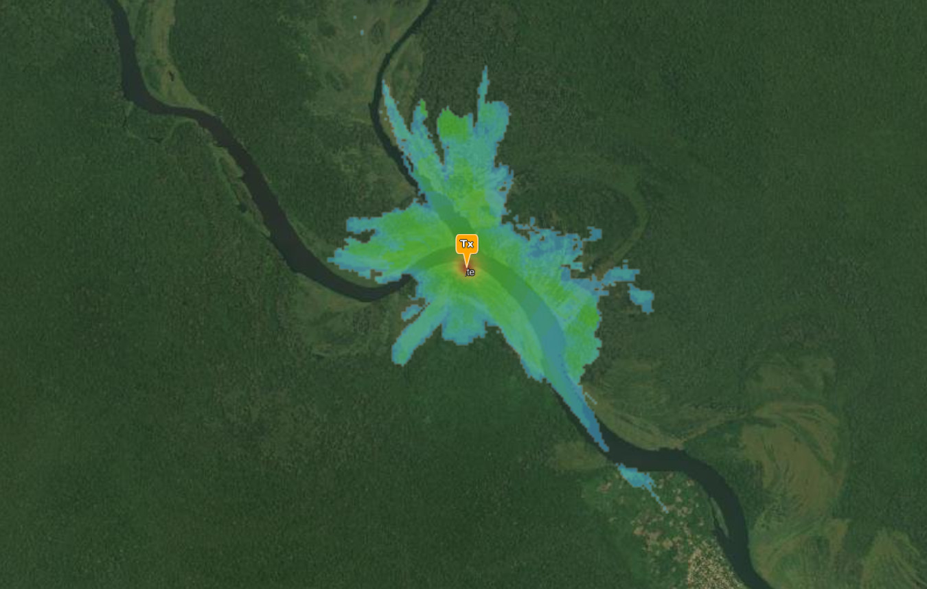
Demo: FM broadcasting (Power)
This is a power problem whereby channels have been separated in frequency but there is interference from neighbouring channels. This is because a signal is shaped with a Gaussian function resembling a bell curve and has power either side of it in the spectrum. The stronger the signal, the more power bleeds into neighbouring channels.
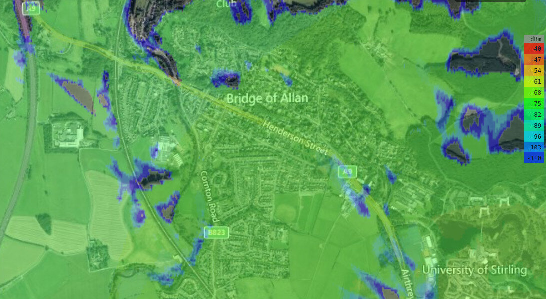
Demo: Microwave link (Bandwidth)
A high power microwave link uses parabolic dishes to focus a high bandwidth beam towards a distant point.
On the path of the link is relatively low power 3GHz cellular system separated in frequency by 45MHz. There is no guard channel so the two signals are adjacent to each other. The directional pattern experiences interference at the edge but is not affected on the main beam.
API demo
We have published a new API demo to demonstrate this scalable capability using vehicles using PMR 446 radios which are being interfered with by other vehicles with different technology in the 446 band.
It uses our Multisite API to model each network for the Signal (Blue) and Noise (Red). When a transmitter, or vehicle in this case, moves, the network is updated and the interference simulated.
Link: https://cloud-rf.github.io/CloudRF-API-clients/slippy-maps/leaflet-interference.html

Documentation
API reference
https://cloudrf.com/documentation/developer/#/Analyse/interference
User documentation
https://cloudrf.com/documentation/04_web_interface_functions.html#interference-analysis
Complete Code example
https://github.com/Cloud-RF/CloudRF-API-clients/blob/master/slippy-maps/leaflet-interference.html
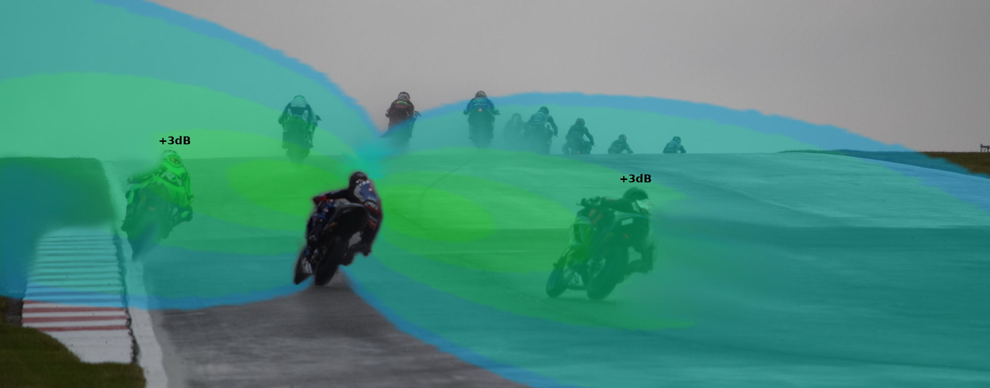


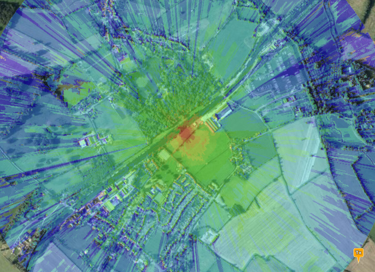

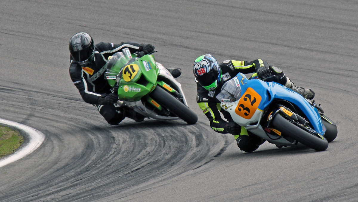 A motorsport customer invited us to a track day to observe a peculiar RF problem…
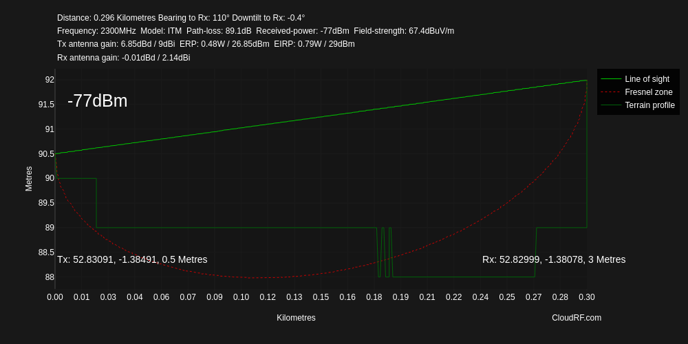
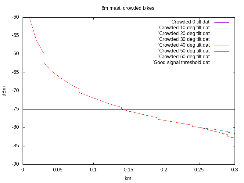
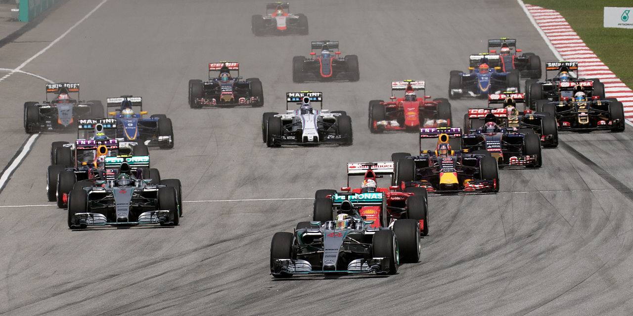
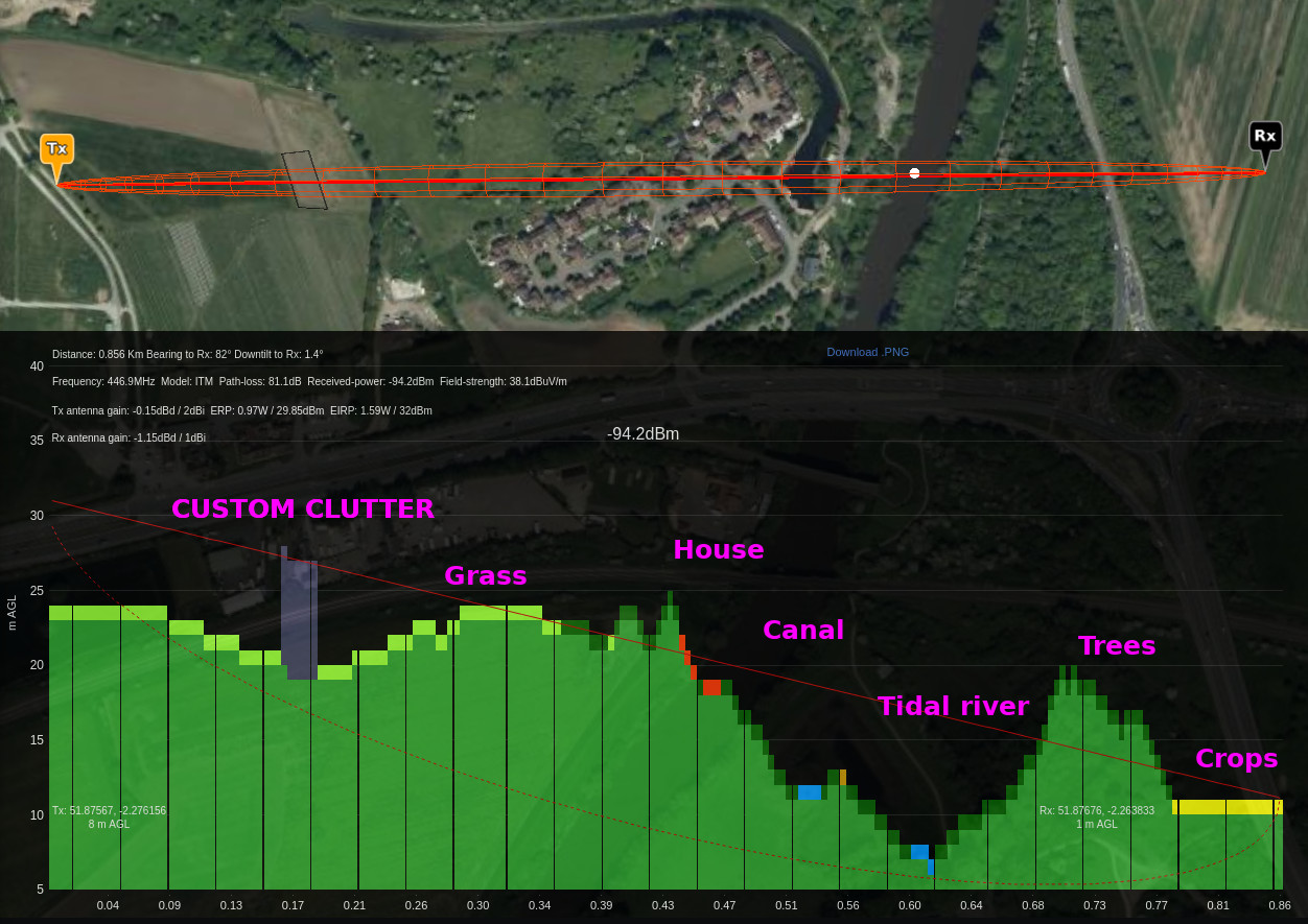
High resolution ‘dashcam’ video feeds have become standard in motorsport with multiple cameras present on vehicles and drivers. Unlike a consumer dashcam, these real-time video feeds use TV broadcasting radio links to relay a signal from the vehicle to the video processing facility via track-side receivers. The problem is Motorbikes with video feeds were experiencing RF difficulty on bends despite being close to high gain receiving antennas. This issue was investigated with the CloudRF API which revealed the following findings:
A motorsport customer invited us to a track day to observe a peculiar RF problem…
High resolution ‘dashcam’ video feeds have become standard in motorsport with multiple cameras present on vehicles and drivers. Unlike a consumer dashcam, these real-time video feeds use TV broadcasting radio links to relay a signal from the vehicle to the video processing facility via track-side receivers. The problem is Motorbikes with video feeds were experiencing RF difficulty on bends despite being close to high gain receiving antennas. This issue was investigated with the CloudRF API which revealed the following findings:
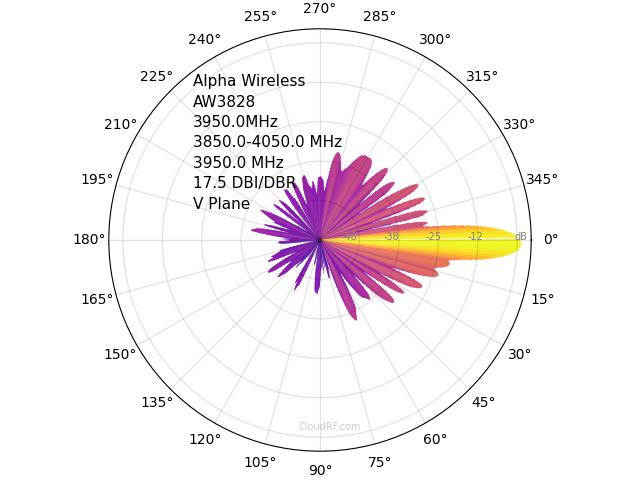
 The antenna on the motorbike is a shark fin, vertically polarised design mounted on the tail of the bike behind the rider.
For the purposes of this investigation the antenna has been modeled with 1dBi gain and and an ERP of 18dBm / 65mW,
equivalent to just under a consumer WiFi router.
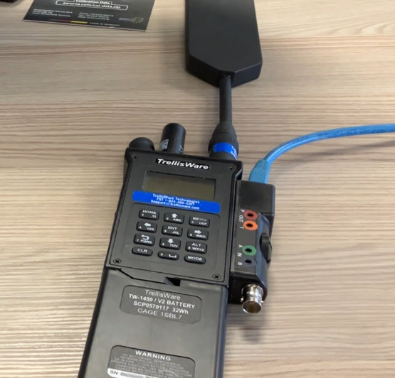
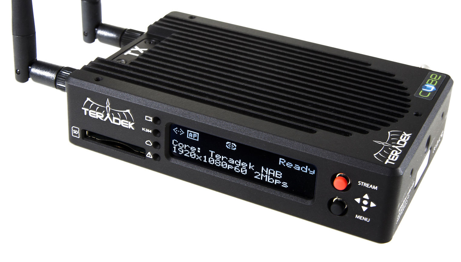
The video broadcast unit is concealed nearby within the bike’s tail with minimal cabling between the antenna for tidiness and maximum efficiency.
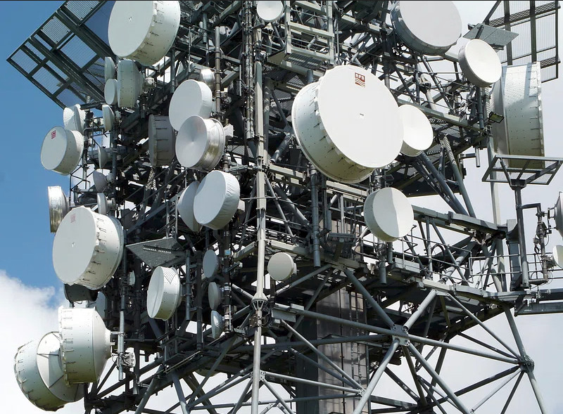
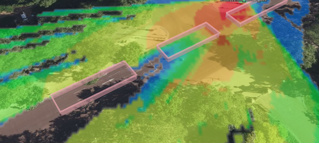
The track-side antennas would be directional antennas with at least 10dBi of forward gain. These would be positioned at key
points on the race track for maximum benefit. The siting of these antennas is where CloudRF is used to test options.
The antenna on the motorbike is a shark fin, vertically polarised design mounted on the tail of the bike behind the rider.
For the purposes of this investigation the antenna has been modeled with 1dBi gain and and an ERP of 18dBm / 65mW,
equivalent to just under a consumer WiFi router.
The video broadcast unit is concealed nearby within the bike’s tail with minimal cabling between the antenna for tidiness and maximum efficiency.
The track-side antennas would be directional antennas with at least 10dBi of forward gain. These would be positioned at key
points on the race track for maximum benefit. The siting of these antennas is where CloudRF is used to test options.