


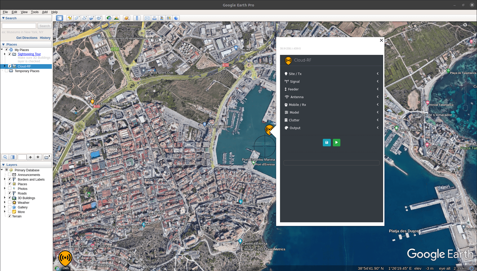
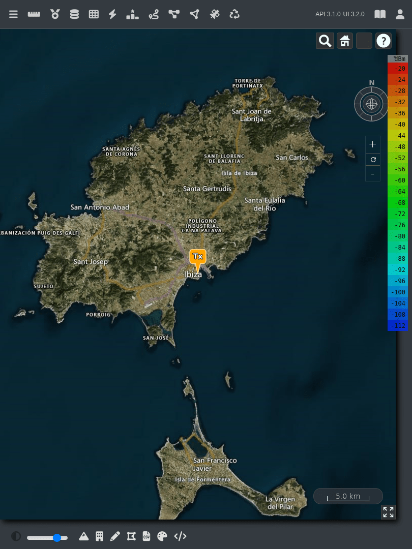
Web Interface
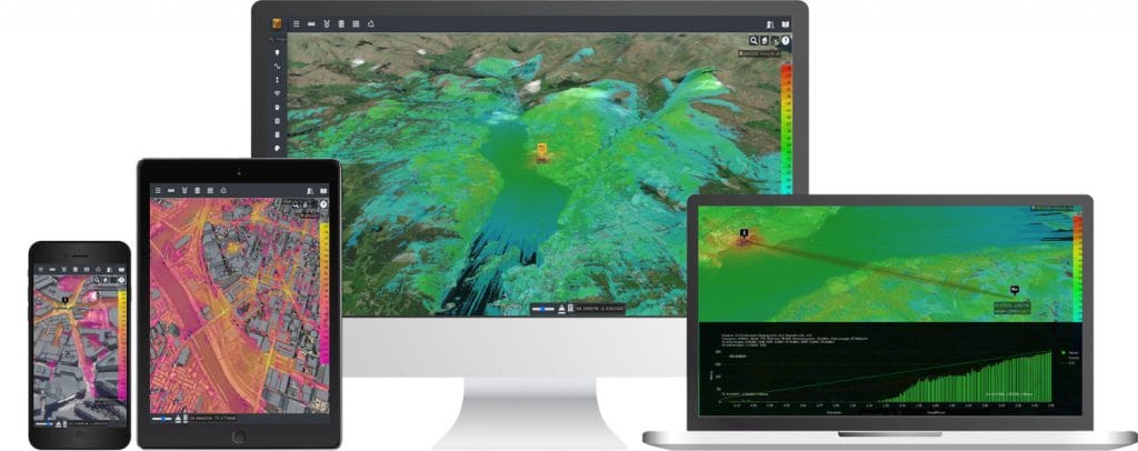
The 3D web interface is the primary user interface for CloudRF. This interface is compatible with desktops, laptops, tablets and even mobile phones.
The interface supports Android, Linux, Mac/OSX and Windows and works best with Google Chrome.
MINIMUM HARDWARE: 4GB of memory, dual core CPU
RECOMMENDED HARDWARE: 8GB of memory, quad core CPU, 1GB GPU
To access the CloudRF 3D Interface:
Click on the Web Interface button on the Home Page.
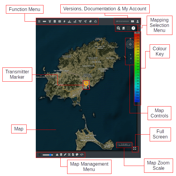
Interface elements
Hot Keys / Keyboard Shortcuts
There are a number of hot keys / keyboard shortcuts which are enabled in the interface which can allow you to manipulate your view/settings without moving your mouse.
You can use the following keyboard shortcuts:
Home- Reset your view to your current Tx marker.Page Up- Zoom out.Page Down- Zoom in.Left Arrow- Pan view left.Up Arrow- Pan view up.Right Arrow- Pan view right.Down Arrow- Pan view down.Control + Left Arrow- Move Tx marker left.Control + Up Arrow- Move Tx marker up.Control + Right Arrow- Move Tx marker right.Control + Down Arrow- Move Tx marker down.Control + Space- Run a calculation.
Transmitter Marker
The Transmitter Marker (Tx) indicates your Antenna Location.

To update your antenna location settings:
On the map, click on the desired location.
The transmitter marker will move to your clicked location.
The location settings under the input menu will be updated respectively.
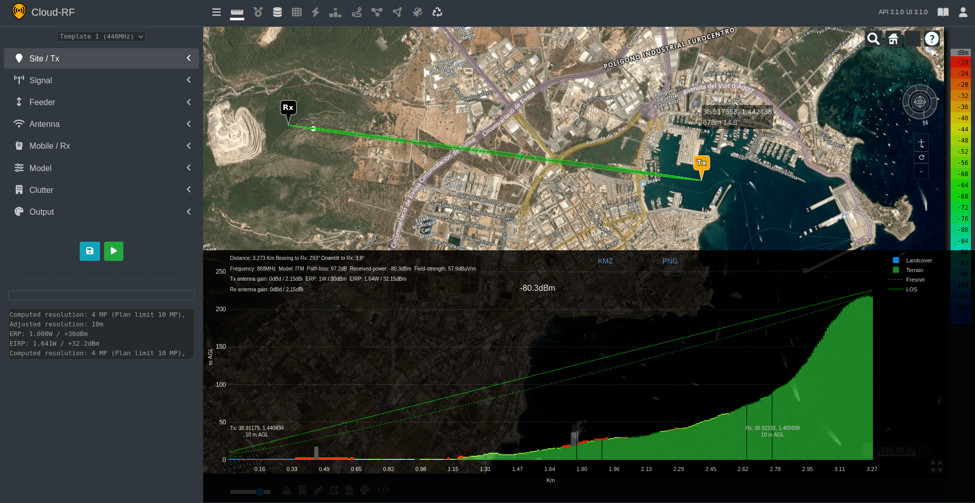
Click on the transmitter marker to view the location parameters of the Transmitter - Latitude and Longitude.
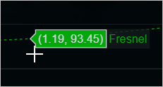
When you have a layer, the information box next to the cursor will display the current co-ordinates, signal strength, distance and angle from the site.
Input Menu
The Input Menu is an accordion style menu consisting of various collapsible sections with input fields. It allows you to focus on several settings which are further grouped into the various categories making it user-friendly.
The fields in the various input menu categories have a Help
icon beside them. To know the details regarding a field, you can click on the Help icon of the respective field.
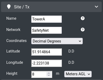
 Site / Tx
The Site / Tx (Transmitter) input menu consists of the settings related to the physical location of the antenna. These settings are relative to the ground and the Name & Parent of the site.
The Site/Tx settings will be of greater importance as your network grows and you need to perform analysis such as the best server analysis.
You can set location in the following two ways:
Manually - You can enter the Location fields (Latitude and Longitude) manually in the respective fields.
OR
Clicking on the Map - You can click on the map and the location fields will be set accordingly.
All the inputs in the form of Decimal Degrees, Degrees/Minutes/Seconds and NATO MGRS are acceptable. The system will make necessary conversions automatically.
Configure the following Site/Tx fields:
Name
Enter the desired unique name for your site.
Network
Enter the network name for logical grouping (as per the cities/area) of your site(s). Minimum length 2 characters eg. “N1”
NOTE: Setting the network is really important as it will help you group and analyse data in the future. Do not use the same value eg. TEST for all your work as you will never find it or be able to run analysis functions on it like the 'network' analysis or 'interference' tools.
Coordinates
Select the desired coordinate format from the drop-down.
Latitude and Longitude - These location fields can be entered manually or set automatically by clicking on the map.
Height
Enter the height (in meters or feet) as either above mean sea level (AMSL) or above ground level (AGL). If using LiDAR and height AGL this is the height above the roof, otherwise it’s relative to the ground. The system’s resolution is 1m minimum so a shoulder mounted radio should be set as 2m and a smart meter on (or below) the ground should be 1m.
The height above mean sea level is relative to the DTM used vs the WGS84 ellipsoid. All sea levels in CloudRF are 0 without tidal adjustments.
The Distance units applying to all heights and radiuses are set here. The default units of the system are metric (m/km)
Choosing Feet will set the distance calculations to Imperial (ft/Mi)
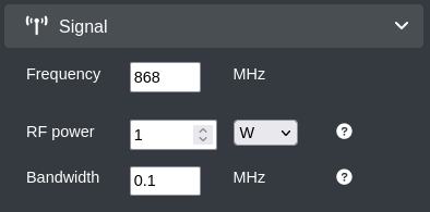
 Signal
The Signal input menu consists of the settings related to the actual radiation.
Configure the following Signal fields:
Frequency
Enter the system frequency (MHz) in the range: 2 to 90,0000 MHz. For a wideband system use the center frequency. For a dynamic system which can go low and high, use the higher value since this will produce the more conservative coverage for planning purposes.
RF Power
Enter the transmitter power (watts or dBm) before feeder loss and antenna gain.
ERP will be auto-calculated and displayed in the output console.
Bandwidth
Enter the channel bandwidth (MHz). Range is 1KHz (0.001MHz) to 200MHz.
Bandwidth will affect Channel Noise and Signal-to-Noise ratio.
Wideband channels will incur increased channel noise and reduced Signal/Noise Ratio.
The system will compensate for wide-band noise by making adjustments to the receiver sensitivity inline with Shannon’s theorem.
WARNING: Bandwidth is ignored for Received power mode (dBm) which is independent of channel noise as it is just the carrier (eg. cw). It becomes very relevant in SNR and RSRP modes, where it will make a significant difference in coverage.
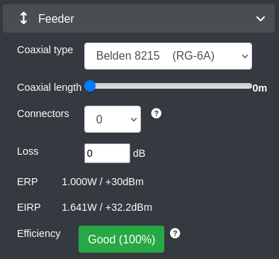
 Feeder
The Feeder input menu consists of the settings related to the cabling & connectors between a transmitter and a radio.
If you have a long feeder, it will absorb power and reduce the efficiency of your system. The most efficient systems have no feeder as the antenna screws onto the radio.
For UHF signals above 300MHz, feeder loss is a significant issue which must be budgeted carefully. A long cable will introduce a lot of loss into a antenna system. They’re also more expensive so get the shorter cable and communicate further!
Coaxial Type
Select the Coaxial standard from the drop-down as per your requirement. The Coaxial Cable used will affect the feeder loss.
This can be safely ignored if the antenna screws directly onto the radio.
Coaxial length
Set the slider to the desired Coaxial length of the cable. The cable length will significantly affect the feeder loss. Even a few meters of coaxial could reduce your system efficiency by 50%.
This can be safely ignored if the antenna screws directly onto the radio.
Connectors
Select the number of connectors from the drop-down as per your requirement.
This will affect the feeder loss.
Loss
Enter the computed feeder loss in decibels. This will typically be in the range: 0 to 15dB.
If the feeder loss is more than 15dB, it indicates that your system is very inefficient and a redesign is recommended.
ERP and EIRP- The dynamically calculated Effective Radiated Power (ERP) and Effective Isotropic Radiated Power (EIRP) will be displayed in the respective fields.
The ERP and EIRP values will change as you manipulate the powers and gains on the interface and will be visible in the corner console.
Efficiency - This label will display the computed efficiency for your system based upon the RF input power and the computed ERP.
 Antenna
The Antenna input menu consists of the settings that lets you choose or build an antenna.
Configure the following Antenna fields:
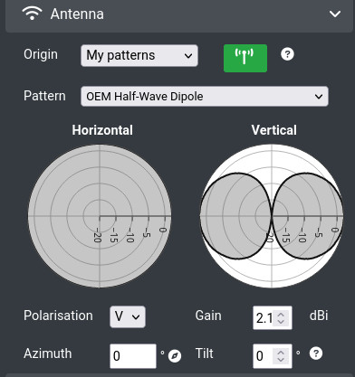
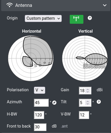
Origin - You can select My Patterns (system template) or Custom Pattern option from the drop-down. A custom pattern lets you build an antenna using beamwidth values in degrees.
If you select the Custom Pattern option:
You can configure the fields:
Beamwidth (horizontal and vertical)
Gain, Front-to-back ratio (use gain if unsure)
Down-tilt relative to the horizon
Azimuth relative to true north. You can use more than one azimuth at a time to simulate the same antenna pointing in different directions. To do this please use a comma-separated list, for example
0,120,240would simulate 3 antennas spaced 120 degrees apart from true North. You can enter up to a maximum of 20 azimuth values. Works with the ‘Area’ API only.
For further information, refer Custom Antenna Pattern Generation topic.
Antenna Pattern database - Explore thousands of patterns in the database and select favourites to appear on your pattern select list.
For further information, refer Antenna archive - searching and favouriting a pattern topic.
Polarisation - You can select Vertical or Horizontal option from the drop-down. Circular polarisation is not yet supported but can be adjusted for using the gains/losses if known.
Gain - Enter the antenna gain relative to an isotropic radiator. A dipole is 2.15 dBi
The peak gain is measured in decibel-isotropic (dBi) and will affect the ERP. For further information, see Feeder input menu.
Azimuth - Enter the horizontal direction of the main lobe relative to grid north (in degree).
You can use more than one azimuth at a time to simulate the same antenna pointing in different directions. To do this please use a comma-separated list, for example
0,120,240would simulate 3 antennas spaced 120 degrees apart from true North. You can enter up to a maximum of 20 azimuth values.You can disable this in path profile mode so it always points along the path by clicking on the Compass icon.

To enable it, click on the Compass icon again.
Down-Tilt - Enter the vertical direction of the main lobe relative to the horizon.
A positive value is towards the earth and a negative value is towards the sky.
Custom Antenna Pattern Creation
You can create custom antenna patterns using the extended options, available when you choose “custom pattern” from the selection.
Custom: Horizontal Beamwidth - Enter the beamwidth in degrees between the half power (-3dB) points on the pattern in the horizontal plane. A cell tower panel might be 120.
Custom: Vertical Beamwidth - Enter the beamwidth in degrees between the half power (-3dB) points on the pattern in the vertical plane. A high gain cell tower panel might be 30.
Polar Plots - The polar plots of the antenna pattern will update as you change the settings so you can see if it looks right.
Custom: Front to back ratio - Enter the Ratio in decibels between the forward and rear gain values of a pattern. Use gain value if unsure.
Ensure you set a positive gain and front-to-back ratio when building a custom pattern.
Antenna database
You can explore antenna patterns in the central database. This is the source for patterns visible when you use the “pop-up” search form in the web interface. The table has columns on the right which may be hidden from view. To reveal them, use the slider at the bottom of the pop up window.
To find and use pattern files:
Click on the green Antenna icon to launch a pop-up form and then click the “Manage My Antennas” hyperlink to redirect.

The Antenna Database screen will appear in a modal window. You can click a link to open it in a new tab.
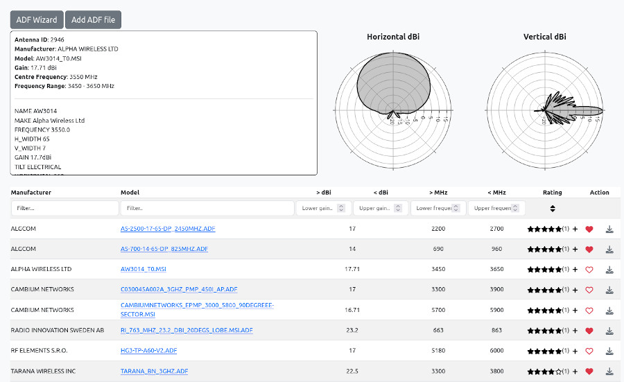
You can either Search and favourite a pattern or upload antenna patterns to add them to your list. For more information on pattern formats and validation, see the antennas section within the reference data section.
Selecting patterns for use
To Search an Antenna Pattern:
Select the Manufacturer from the drop-down.
Select the Model by typing characters from the name eg. DIP..
For Favouriting an Antenna Pattern:
In the ‘Action’ column on the right of the table, click on the heart
 icon of the pattern.
The icon will turn red
 indicating that the pattern has been short-listed. It will appear in your antennas list after re-loading the user interface.
Antenna ratings system
Antenna patterns vary in quality. You can provide feedback on good patterns which helps your team find them quicker since they are ranked by score. Click the rating stars and provide a score and a reason.
Removing patterns
At the time of writing, patterns can only be removed by emailing support@cloudrf.com with the name and ID number(s). A delete function is scheduled.
Antenna pattern validators
An ADF validator is here.
A multi-format conversion wizard is here.
To upload a new antenna pattern,
Click ‘Add ADF file’ to open the form and upload your file:
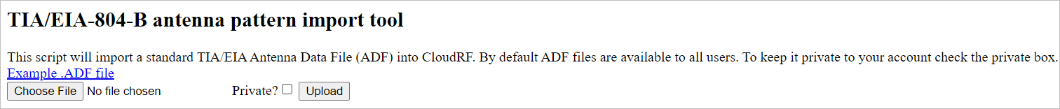
Click on Choose File button to browse and select the desired file to upload.
If you wish to keep the uploaded pattern file private to your account, select the Private? checkbox. Be aware that the OEM will still be public.
Click on the Upload button.
 Mobile / Rx
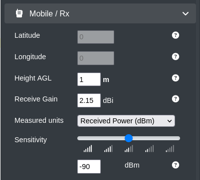
The Mobile / Rx (Receiver) input menu contains settings for the remote end of the link. This could be a mobile outstation, a customer or a vehicle.
Configure the following Mobile/Rx fields:
Latitude and Longitude
These location fields will be disabled by default.
To enable the fields, you can click on the Path Profile tool  icon on the Function Menu.
You can set the receiver location by one of the following ways:
Click on the map. The location values will be set automatically.
Enter the values manually if you know the GPS or map locations.
Height
The height (surface model) in meters or feet. The Height units (metres/feet) and mode (AMSL or AGL) can be set under Site/Tx Input Menu in the Height field. For example: If the surface model is LIDAR that includes a 30m building and your mobile station is 4m on the roof then the Height AGL will be 4m.
If LIDAR is not present the height should be 34m AGL, and if height units above sea level (AMSL) are used, with a ground height of 100m, then the height should be 134m.
For a handheld or shoulder mounted radio, you should use a height value of 2m as the system’s minimum resolution is 1m. Using 1.5m would be rounded to 2m at the API. Using 1.4m would give a more conservative prediction as it would be rounded down to 1m.
Receive Gain
Enter the receiver gain in dBi. This is the combined receiver and antenna gain. The receiver gain considers the antenna, receiver noise and (receive) feeder loss. For example: If the receiver has a 3dBi antenna and a 3dBi receiver noise figure, the Receive gain would be 0 dBi.
For a Mobile Phone, you should use a gain value of 0dBi. The actual performance varies by band, so a phone may have 1dBi gain for GSM900 but 0dBi for UMTS2100. Choose the lower value if you are unsure.
Measured units
Select the output units option from the drop-down as per your requirement. CloudRF has support for a wide range of different measured units. The units must correspond with the selected colour key if performing area coverage plots.
Path Loss (dB)
Discounts transmitter power. Useful for selecting equipment for a link as this will give you an idea of what transmit power you will need to overcome the path loss.
Received Power (dBm)
Default units for consumers and operators. This is for modelling the carrier/signal only so it discounts noise floor and bandwidth and is used widely in IoT / LPWAN, WiFi and consumer applications. For full-bandwidth modelling see RSRP below.
Field Strength (dBµV)
Decibel-micro-volt-per-meter. Used for broadcasting and specialist power measurement. Has a relationship with received power so you can convert one to the other.
dBuV = dBm + 90 + 20log(ohms)
Signal to Noise Ratio (dB)
SNR considers noise floor and bandwidth. Used for MANET, Radar, cellular, 4G and 5G technologies. If you have noise data for the noise API, you need to be using SNR.
Bit-Error-Rate (BER)
Uses modulation curves and the noise floor to dynamically compute an SNR value as a threshold. Used for SATCOM and microwave links.
Pick your modulation schema from the list, then select the Bit-Error-Rate. The system will use these inputs, in conjunction with the noise floor to apply the appropriate SNR as dB.
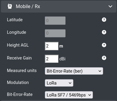
LoRa spreading factor (SF) can be applied by choosing “LoRa” as the modulation. SF7 gives the best throughput but has a higher SNR requirement. Conversely, SF12 has the best range at the cost of throughput.
Reference Signal Received Power (dBm)
RSRP considers bandwidth. This is widely used in cellular systems with variable bandwidth like 4G (LTE) and 5G-NR and is always a lower figure than the received power (dBm) for the same signal.
Best Site Analysis (%)
The output for BSA is a percent (%) denoting relative site efficiency. Please note that BSA is only supported with Best Site Analysis calculations.
Sensitivity
Set the sensitivity slider to define the sensitivity of the mobile station in units corresponding to the measured units.
WARNING! SET WITH CARE
Use -90dBm if unsure.
A mobile phone’s sensitivity is between -100dBm and -115dBm. Setting the sensitivity too low (eg. -120dBm) will result in an unrealistic BIG prediction. Be aware also that phones can report signal strength as RSRP or received power yet the difference between the two is significant depending on bandwidth. RSRP is the lower value.
IoT protocols like LoRa / LPWAN can theoretically operate down to -140dBm but this is under ideal conditions. To simulate man-made noise, add a margin of at least 10dB so your threshold is at least -130dBm.
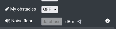
Noise floor (SNR and BER units only)
Since v3.9, noise floor has been moved to the environment menu. Enter the local noise floor value in dBm. It is used in conjunction with the required SNR to establish the sensitivity.
The system will help you with a thermal noise value (Johnson-Nyquist) based upon your chosen bandwidth but for best results, you need to measure the noise in your area and enter a measured value.
Since v3.9, you can enter noise in real time through the noise API. If you have live measurement data, you can then ensure that your planning matches the reality, whatever the reality may be. Click the network icon next to noise to enable “database” mode instead of system default, or guessed, values.
 Model
Model
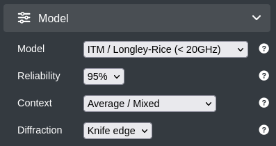
The Model input menu consists of the settings related to the Propagation Model.
Configure the following Model fields:
Model - Select the Propagation model from the drop-down as per your requirement. Some empirical models like Hata and SUI have minimum frequencies and heights. This is enforced as these models will only be accurate if used within their parameters.
Use the ITM model if you are unsure. This is used by the FCC for general purpose applications and is the most advanced model here where VHF/UHF diffraction is present.
Model |
Purpose |
Frequency Range |
Minimum Tx Height |
|---|---|---|---|
COST231-Hata |
Cellular |
150 - 2000 MHz |
3m |
Egli VHF/UHF |
General Purpose |
2 - 1500 MHz |
0.1m |
Ericsson 9999 |
Cellular |
150 - 1900 MHz |
3m |
ITM / Longley Rice |
General Purpose VHF/UHF |
2 - 20,000 MHz |
0.1m |
ITU-R P.525 (Free Space) |
Reference model |
2 - 90,000 MHz |
0.1m |
ITU-R P.529 (ECC33) |
VHF/UHF |
700 - 3500 MHz |
0.1m |
Line of Sight |
Any |
Any |
0.1m |
Okumura-Hata |
Cellular |
150 - 1500 MHz |
3m |
RADAR (ITU-R P.525 w/RCS) |
RADAR |
2 - 90,000 MHz |
0.1m |
SUI Microwave |
UHF/SHF |
1900 - 11,000 MHz |
3m |
WARNING: The ITU-R P.525 model is a simple reference model. It will provide a very optimistic prediction (eg. +20dB gain) unless you temper it with losses elsewhere.
WARNING: When selecting the “Line of Sight” model knife edge diffraction should be disabled.
RCS - When you select the RADAR propagation model you will also be prompted to specify a RADAR Cross Section (RCS) value. This value is used to descrive an object’s reflective surface and is measured in square meters (m2). In general, the larger the object the higher its RCS value. Some examples are listed below:
Bird:
0.01m2Small drone: <
0.04m2Human:
1.0m2Jet aircraft:
2-6m2Cargo aircraft:
100m2Automobile:
100m2Coastal vessel:
300-4000m2Container ship:
10,000-80,000m2
Reliability - This field enhances a model with a 10dB fade margin. You can select the reliability percentage as per your requirement.
99% indicates a conservative ‘high confidence’ prediction (+9.9dB path loss)
95% is the default set value.
50% is an optimistic “sunny day” prediction (+0dB path loss)
Context - Select the context of the model from the drop-down as per your requirement. Many models have environmental variables which provide different outputs.
Tip: For a conservative output, select Conservative/Urban as the option. Else, keep the default Average/Mixed option and use the reliability for tuning.
Diffraction - Diffraction will show coverage beyond an obstacle. The radio shadow size will vary by frequency and the obstacle distance/height with a low frequency having a low angle of diffraction. The recommended value for frequencies below 6GHz is ON / Knife edge.
 Environment
The Environment input menu consists of the settings related to the system and custom clutter. For more information see the clutter reference.
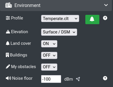
Profile
Select the regional profile from the drop-down as per your requirement. If no profile has been created you will be shown Minimal.clt. See the clutter manager section below for how to manage clutter profiles.
Elevation
Select the digital elevation model.
Surface / DSMwill use a rough surface model or LiDAR if it is available. Heights are relative to rooftops.Terrain / DTMwill use a bare earth model so heights are relative to the ground.
Land cover
Select the Land cover mode from the drop-down as per your requirement.
OFFwill just use terrain data.ONwill add system 10m landcover.
Buildings
Select the Buildings mode from the drop-down as per your requirement.
OFFwill just use terrain data.ONwill add a buildings layer to the surface model (Coverage varies by region)
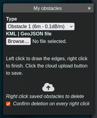
My obstacles
Choose to enable your custom clutter. Your items, such as a building, will be placed upon the terrain by default and can be used alongside land cover. To use this function, you must have clutter items saved to your account. See the clutter reference for more.
OFFwill not add any custom clutter.ONwill add custom clutter on the chosen elevation model. Use with care.
Clutter Manager 
The clutter profile manager can be opened with the green-tree clutter manager button.
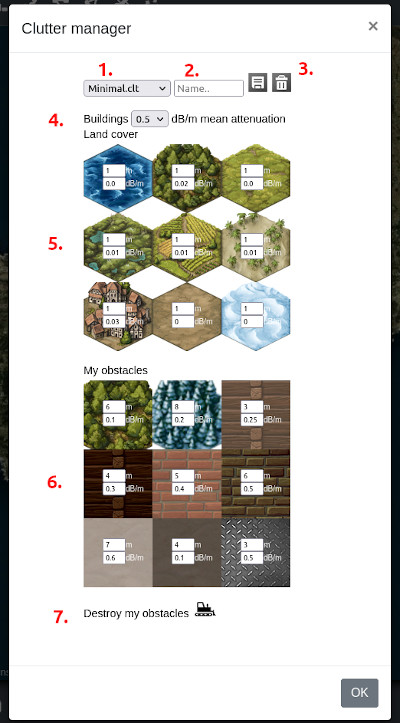
Selected Profile
Save new profile as name
Save and delete name listed in 2.
Building attenuation
Land cover types
My obstacle (clutter) types
Delete my obstacles
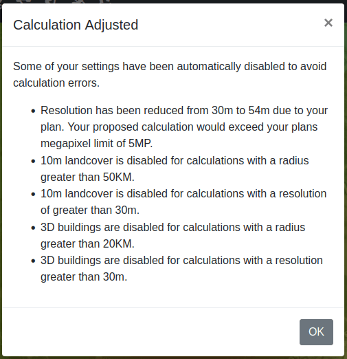
Clutter Restrictions
Please note that there are restrictions in place on the public API which will protect it from being run with unnecessary or bogus values. The rules which are enforced on the API are:
Enabling 10m landcover on calculations with a radius greater than 50km.
Enabling 10m landcover on calculations with a resolution greater than 30m.
Enabling 3D buildings on calculations with a radius greater than 20km.
Enabling 3D buildings on calculations with a resolution of greated than 30m.
In such circumstances you will receive a “Calculation Adjusted” message with your response indicating what has been adjusted or disabled from your request.
Clutter attenuation
The Clutter Attenuation is a nominal value measued in decibels per metre (dB/m) for an obstacle, not the material itself, based on the principle of a hollow composite house or a forest with uniform gaps between trees.
For example: A 10m house with 2x 7dB brick walls and 2x 3dB partition walls would have an average of 2.0dB/m. This would be very conservative due to the Windows which permit signals, at the right angle ;), so by using a quarter of this we get 0.5dB/m which is a better nominal value for “a house”.
No two houses or forests are the same so results will vary by town and country. For best results, calibrate a profile based upon street level measurements. Taking measurements from up high will miss clutter and likely provide an optimistic profile.
The following values are used in the minimal template. For codes, see the clutter reference.
1	1	0.0
2	5	0.05
3	1	0.0
4	1	0.02
5	1	0.05
6	2	0.05
7	1	0.03
8	1	0
9	1	0
10	0	0
11	6	0.1
12	8	0.2
13	3	0.25
14	4	0.3
15	5	0.4
16	6	0.5
17	7	0.6
18	8	0.7
19	3	1.0
Building attenuation
Building attenuation is a separate value to the 9 land cover attenuation values as it is a distinct layer. Like other types, it is a nominal attenuation value measured in dB/m and is applies to the whole of a building, not just the walls.
For example, a house with 2x 10dB thick walls, measuring 8m deep, will have a value of (2 x 10) / 8 = 2.5dB/m. In reality, a house has windows which allow signals to pass. Depending on the glass, this could be as low as 2dB so a glass house becomes (2 x 2) / 8 = 0.5dB/m. Taking an average of the two gives 1.5dB/m.
For celular networks, building attenuation is significant. Most of the signal behind a house is diffracted from the roof, so going away from the house to the end of the garden will boost your signal.
Value |
Building type |
|---|---|
0.1 |
Timber |
0.2 |
Light brick |
0.3 - 0.5 |
Brick / Concrete |
0.5 - 0.8 |
Concrete |
0.8 - 4.0 |
Concrete / Metal |
Saving and deleting profiles
Enter the name for your profile eg. POLAND and click the save button. To delete, enter the full name of the profile plus the file extension eg. POLAND.clt then click the delete button.
Noise floor
Since v3.9, noise floor has been moved to the environment menu.
Enter the local noise floor value in dBm. It is used in conjunction with the required SNR to establish the sensitivity when using SNR, RSRP or BER units only.
NOTE: Noise floor is ignored in received power mode (dBm)
The system will help you with a thermal noise value (Johnson-Nyquist) based upon your chosen bandwidth but for best results, you need to measure the noise in your area and enter a measured value.
Since v3.9, you can enter noise in real time through the noise API. If you have live measurement data, you can then ensure that your planning matches the reality, whatever the reality may be. Click the network icon next to noise to enable “database” mode instead of system default, or guessed, values.
To push in noise data, send a POST request to the https://api.cloudrf.com/noise/create endpoint or paste CSV data into the hosted form at https://cloud-rf.github.io/CloudRF-API-clients/integrations/noise/noise_client.html
 Output
The Output input menu consists of the settings related to the system output.
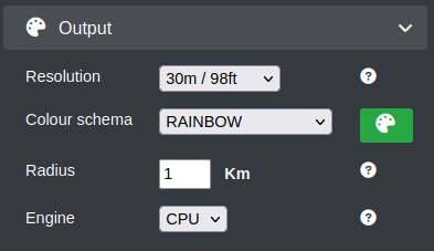
Configure the following Output fields:
Resolution
Select the desired resolution from the drop-down as per your requirement. Make sure that the resolution when combined with the radius to compute a mega-pixel value, is within your plan limit.
2m is not recommended unless you know that the city or area supports this data via LiDAR.
TIP: 20m presents a much better compromise for accuracy in most countries due to proximity to the underlying surface model and the use of 10m landcover.
Colour Schema
Specify how the produced calculation will be coloured based on a selected colour schema.
Please Note that schemas here listed are based on your selected “Measured Units” value in the “Mobile / Rx” menu. If you are looking for a schema which isn’t listed here then it is likely caused by the schema belonging to a different measured unit eg. dB vs dBm
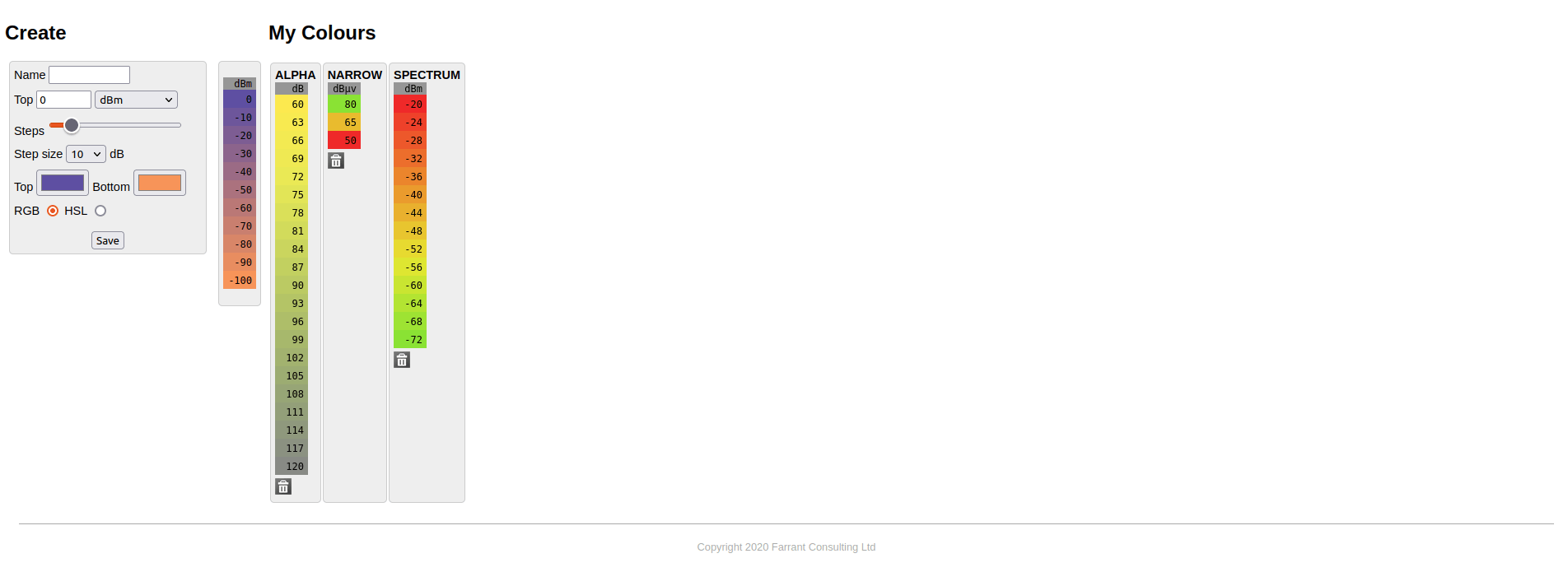
You have a list of system-default colour schemas to choose from, however if these do not fit your use-case then you can also create your own colour schema by clicking on the colour palette icon.

When you do this you will be presented with the My Colours screen. Here you can build a colour schema.
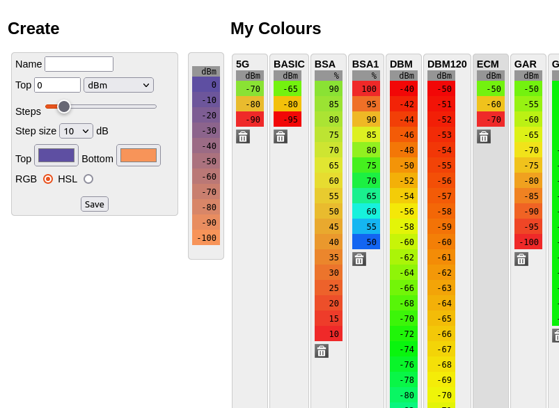
Choose your units eg. dBm
Give it a name eg. GREEN2RED
Choose a sensible top value. -30dBm is a good place to start.
Choose a step size and steps with the slider.
Choose your colours - this is what you came for
Choose a colour schema. HSL is recommended for a dynamic rainbow range.
Radius
Enter the desired radius in the units as chosen in the transmitter menu. This value is used with resolution to compute mega-pixels which are displayed in the corner console. For example: 5km radius calculation at 2m resolution would result in 25MP image. Similarly, 5km at 10m = 1 MP.
NOTE: Do not request an excessive radius/resolution eg. > 32MP. For example, a 20km radius calculation at 2m resolution would create a 400(!) megapixel image which would crash any image processing software and web browser - if you generated it. There are restrictions in place on the API to enforce limits.
Target radius |
Recommend resolution |
Megapixels |
|---|---|---|
1km |
1m |
4MP |
2km |
2m |
4MP |
5km |
10m |
1MP |
10km |
10m |
4MP |
20km |
20m |
4MP |
30km |
30m |
4MP |
500km |
180m |
32MP |
Engine
Choose your desired processing engine to produce the calculation. You have a choice between CPU or GPU.
CPU is our most robust and tested processing engine “SLEIPNIR”. It uses a traditional computer CPU in the background to run through your calculation. This has the benefit of being well matured and tested and so your results will be as accurate as the inputs you specified.
GPU is our newest processing engine. It uses a graphics card so is 20 times faster than CPU processing. It can do diffraction, attenuation and the same propagation models as the CPU engine with the exception of the ITM model which is under development (September 2023).
GPU Engine
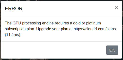
In order to make use of the GPU processing engine you will need to have either a gold or platinum subscription plan, or an enterprise server. If you do not have either then you will receive a forbidden message for the reponse.
When you select “GPU” from the “Engine” dropdown a section will show at the bottom:
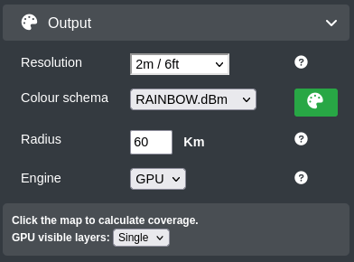
This indicates that you are in GPU mode and you should note a few things:
You can now click on the map to run a calculation. The GPU engine is so fast that a progress bar is not required and so the classic green “Calculate” button is hidden.
You can change the GPU visible layers:
Single means that only one GPU calculation will be kept on the map at a given time.
Many means that you can have as many GPU calculation layers on the map as you wish. However, please note that the GPU engine is fast and so it can very quickly use up your browser resources if you are adding many layers. You can manage layers in the same way as you do for CPU calculations in the top right.
Colour Palettes
You may find that the system-defined colour schemas do not meet all of your requirements and so to resolve this CloudRF has functionality to build your own colour schema with your own colours, units and limits.
To create custom colour pattern:
Select the colour schema by clicking on the Manage My Colours
icon. This button can be found in both the “Output” menu and also in the “Account Information” modal.The My Colours screen will appear in a separate tab on your browser.
Note When you load this manager you may have no colours to the right under the “My Colours” heading. This is normal, as you have not yet created any colours.
You may create a customised colour pattern by using the form on the left.
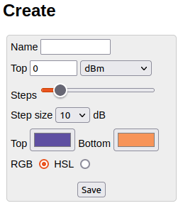
Name is the name of your custom colour schema.
To edit an existing pattern, enter the colour pattern name here. You may edit the fields as per your requirement.
Top is the top-most value of the colour pattern. Use -30 for a received power schema.
As part of Top you should select the unit under which your colour pattern will be used. Your pattern can only be used with that measured unit. If you require patterns for other units then you should create those separately.
dB - Decibels
dBm - Decibel milliwatts
dBuV/m - Decibel microvolts per meter
% - Percentage coverage for best site analysis calculations
BER - Bit-error-rate
When selecting BER you will see a second dropdown get created which asks you for your modulation.
RSRP (dBm) - Reference signal received power in decibel milliwatts
Steps is the number of steps/buckets you wish to be displayed in the colour pattern.
Step size is how spaced apart each step/bucket is, for the total number of Steps.
Top and Bottom are the colours you wish to use for the top and bottom of the colour pattern.
RGB and HSL correspond to the colour format to be used between the steps. RGB (red, green, blue) are more computer-readable. HSL (hue, saturation, lightness) are more human-readable and will provide a better dynamic range.
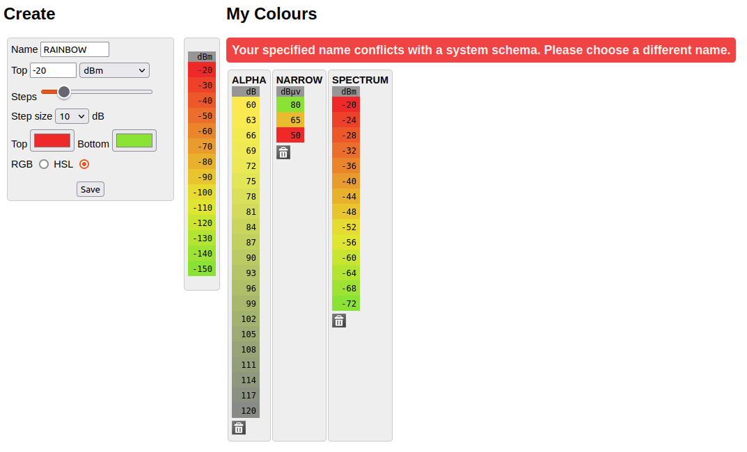
As you adjust the settings from the form the colour schema will be built on-the-fly to the right of the form.RAINBOW
Once you get the colour schema to a stage which you are happy with then you can click on the Save button where your colour schema will be attempted to saved to your profile.
If there are any problems then you will received a validation message towards the top of the screen.
If your colour schema could be created successfully then you will be notified with a success message and your new colour schema will be displayed on the right under the “My Colours” heading.
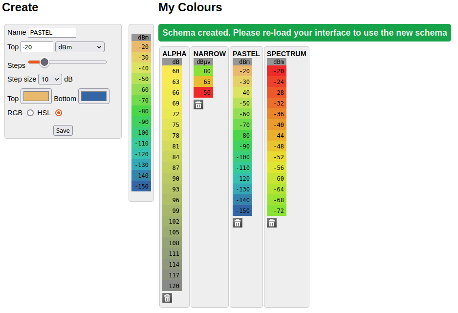
You can now return to the web interface and your colour schema will be present in the “Colour Schema” dropdown on the “Output” menu, as long as you have the correct “Measured Units” selected from the “Mobile / Rx” menu which matches your new colour schema.
Save and Run Buttons
After configuring the Input Menu, you can Save and Run the configuration by clicking on the respective button.
These buttons are displayed below the Input Menu.
 Save
Save
Save button lets you create a template with all your configured settings that you can reuse later whenever required.
For further information, refer Templates topic.
 Run
Run
Run button will execute a coverage calculation using your configured settings.
The execution may take several seconds depending on the resolution and the radius. The Progress Bar will be displayed in this case.
In case there are errors in the configuration, the respective error dialog box will appear.
Make the necessary corrections and re-run the updated configuration.
After successful execution, the Site name (Network name) field will be displayed in the Output Console.
For further information, refer the Output Console topic.
Templates
Templates allows you to quickly apply settings from a saved/custom or system-defined configuration.
Templates are useful in a shared account where an Engineer might prepare the template(s) and a sales person might use them to qualify customers.
Custom Templates
To manage your custom templates:
Configure the Input Menu as per your requirement.
Click on the Save
button.The Manage Your Templates dialog box will appear.
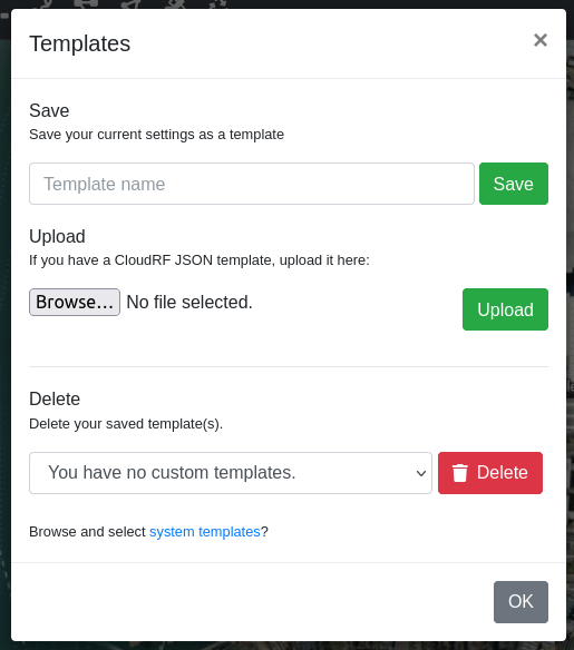
Saving a Custom Template
To save a custom template:
After configuration in the Input Menu, click on the Save
button.In the Manage Your Templates dialog box.
In the Template Name field, enter the desired name of your custom template.
You can give a user-friendly name, for example: “Radio X”.
Click on Save button.
The created Template will be displayed under My Templates drop-down. All custom templates will be prefixed with the words “Custom”.
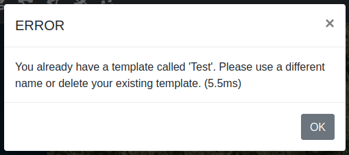
If your settings have any issues when you attempt to create a tempalte then you will be notified via a modal window.
An example of a bad template upload is below.
Uploading a Custom Template
You can upload templates directly into the system. This is useful if you would like to create and share your own templates.
To upload a custom template:
Click on the “Browse…” button to search through your local filesystem to find the JSON template which you wish to upload.
Click on the “Upload” button.
The template will be uploaded and validated. If your template has all of the required fields in the correct formats then your template will be made available to use in your user account. If your uploaded template has any problems then you will be notified via a modal window.
An example of a bad template upload is below.
Deleting a Custom Template
To delete a custom template:
Click on the Template save
button.In the Templates dialog box.
In the Delete field, select the Template Name that you wish to delete.
Click on Delete button.
The deleted Template will be removed from the My Templates drop-down.
System Templates
System Templates provide a list of pre-built templates, built from product data sheets.
To manage your system templates there are 2 methods:
Click on the “Templates” button
 in the manager in the “Account Information” modal.
Click on “system templates” in the “Templates” modal.
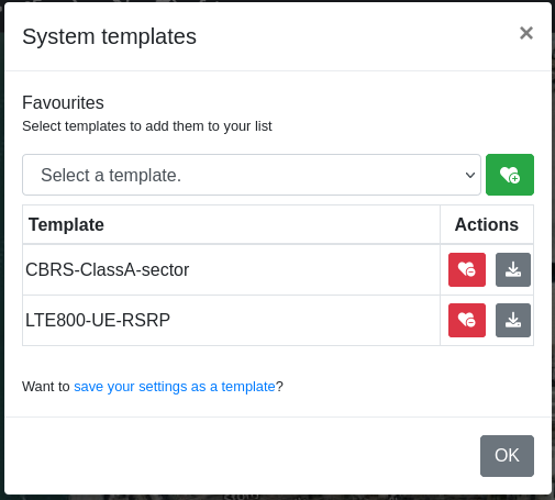
Favouriting System Templates
To add a system template to the templates dropdown you can find the template you wish to favourite from the select list, then click the favourite button  .
.
The chosen template will then be shown in the list below where you will have the option to either remove it or download the system template as a JSON file.
When you have favourited a system template it will be populated into the My Templates dropdown and will be prefixed with the words “System”.
Unfavouriting System Templates
To unfavourite a system template click on the “Unfavourite” button  .
.
This will remove it from the list of templates at the bottom of the system-template manager, but also from the My Templates dropdown.
Downloading System Templates
To download the content of a system template click on the “Download” button  .
.
This will download directly to your browser the raw content of the template in a JSON file. You may edit this in any text editor. A reference for the values is linked in the header of each file.
Download Templates
You can download the raw content of a template directly to your browser by clicking on the download button to the right of the dropdown.
This will download the template as a JSON text file. This will contain all of the settings related to applying that template.
You can download both custom and system templates in this way. You may edit this in any text editor. A reference for the values is linked in the header of each file.
Template privacy and copyright
A template file is potentially sensitive as it can describe equipment configurations and performance. User templates are stored in a user’s private folder with a random cryptographic hash to prevent file guessing attacks. The copyright for a created template belongs to the customer and (JSON file) sharing is actively encouraged.
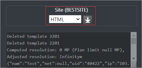
Output Console
The output console provides the useful feedback related to the settings, errors, API inputs and API outputs as you use the CloudRF tool.
The Effective Radiated Power (ERP) and the computed resolution (in mega-pixels) will be printed in this console as you adjust the settings so that you can keep an eye on the same.
As an area calculation processes, you will see periodic updates in the console from the SLEIPNIR propagation engine.
When you submit a calculation for processing, all the API parameters will be displayed here. If you are a developer, you can directly copy paste this to use it in your code.
To do so:
Click on the Run button for execution, the Site name (Network name) field will be displayed in the Output Console.
Select the file format in which you wish to download the configuration settings file.
Click on Download
 icon.
icon.
System Version
In the top right corner of the interface indicates the current version of the API and UI which you are using. The discrete green / amber / red light to the left denotes connectivity to the backend processing service / API. Green is good, amber is connected but the API has been under a sustained load for more than a minute and red is API unavailable.
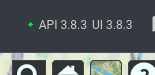
You can click on either of the API or the UI which will open up a modal window in the interface which will give you a full changelog of what has changed in the version you are using.
 Documentation
To refer to the 3D Interface Documentation:
Click on the Documentation
button located on the top right of the interface.
 Account Information
You can view information about your account by clicking on the Account Information icon located on the top right of the interface.
When you click on this a modal window will be opened which will contain various information.
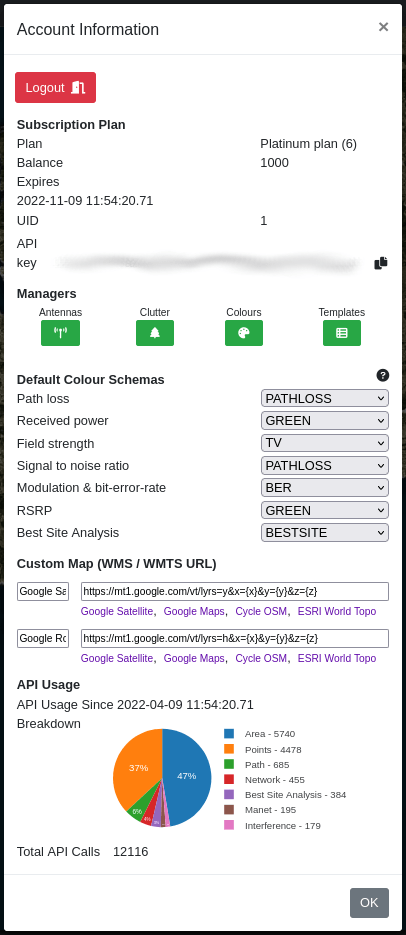
Logout is used to log you out from the system.
Subscription Plan contains information about your current subscription details.
Managers are buttons to other tools to allow you to customise your system settings.
Default Colour Schemas allows you to specify which colour schemas are selected by default for each of the available measured units.
Custom Map lets you define either WMS or WMTS URLs which can be used in the UI to set your own custom map service.
API Usage gives a breakdown of your API usage over the period of your subscription.
Logout
You can logout from the interface by clicking on the logout button at the top of the “Account Information” modal.
Subscription Plan
Details about your current subscription plan are listed in the “Account Information” modal. Such information includes:
Your plan name.
Your account balance.
The expiry date of your current subscription.
Your UID.
Your API key, with a quick copy button.
Managers
CloudRF by default may not have the required settings or customisations which you require, and so we include a number of different managers to allow you to build elements yourself.
- Manage My Antennas allows you to import your own antenna patterns. Please consult the antenna management reference for further details.
- Manage Clutter Profiles allows you to define the height and attenuation of environments. Please consult the clutter profile management reference for further details.
- Manage My Colours allows you to build your own colour schemas. Please consult the colour management reference for further details.
- Manage System Templates allows you to manage your favourite system templates which can be quickly selected from the My Templates dropdown. Please consult the templates reference for further details.
Default Colour Schemas
With CloudRF we support a number of different measured units. As such there are limitations to using some measured units with some colour schemas. The utility in this section allows you to easily select a default colour schema for a number of different measured units:
Path loss
Received power
Field strength
Signal-to-noise ratio
Modulation and bit-error-rate
Reference Signal Received Power (RSRP)
Best site analysis
The schema which you choose here will be the default when you switch your measure unit in the “Mobile / Receiver” menu.
Custom Map
The Custom Map URLs let you define your own map tile servers which can then be used in the interface and selected on the imagery icon. This is useful if the default map layers provided do not meet your own particular needs or requirements.
API Usage
API usage will give you a breakdown of your usage since your subscription was created. This includes a chart and full breakdown of the number of each individual API requests.
Mobile Operation
The CloudRF 3D Interface can be easily accessed on your mobile phone.
The following UI will be displayed on your mobile phone, with a collapsed menu:
3D Interface Elements - Mobile View
Expand/Collapse
The Expand/Collapse  button of the Function Menu lets you expand or collapse the Side Menu consisting of Templates, Input Menu and Output Console.