


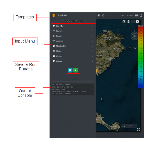
Web Interface Map
Mapping Selection Menu
The Mapping Selection Menu is a set of key mapping functions located on the top-right of the interface.
Mapping Selection Menu Elements
 Address search
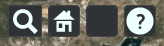
The search tool lets you search an address, landmark, geocode or postcode / ZIP code.
Click on the Search
icon to open the search box.Type the desired address or landmark you wish to search on the map. You will be prompted with different suggestions.
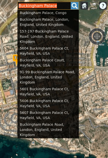
Select your chosen address/landmark/geocode/postcode and the map will be moved to the location.
 View Home
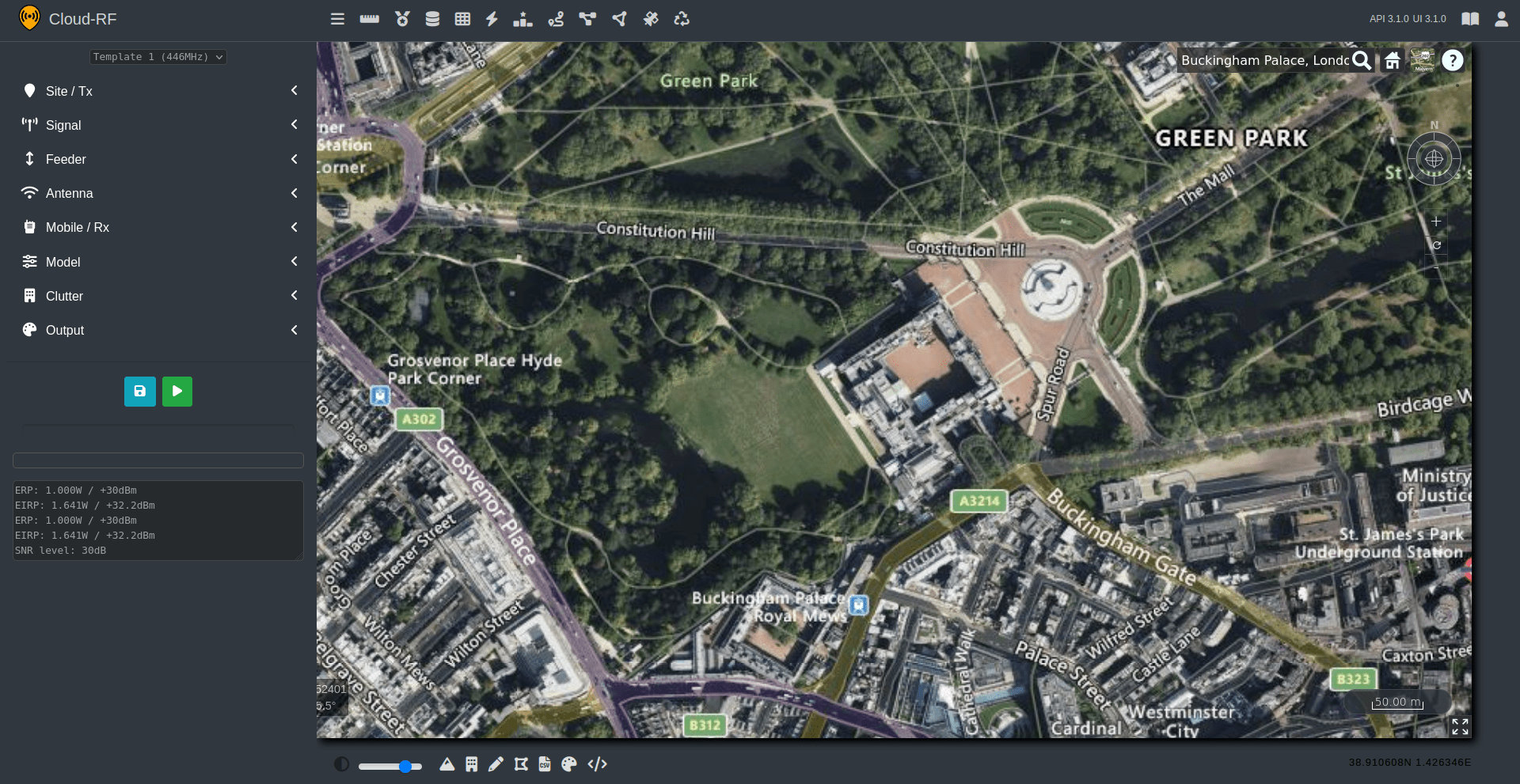
The View Home button is used to reset the interface back to an overview of the whole of the Earth.
Click on the View Home
icon.The following screen will be displayed.
 Choosing Imagery
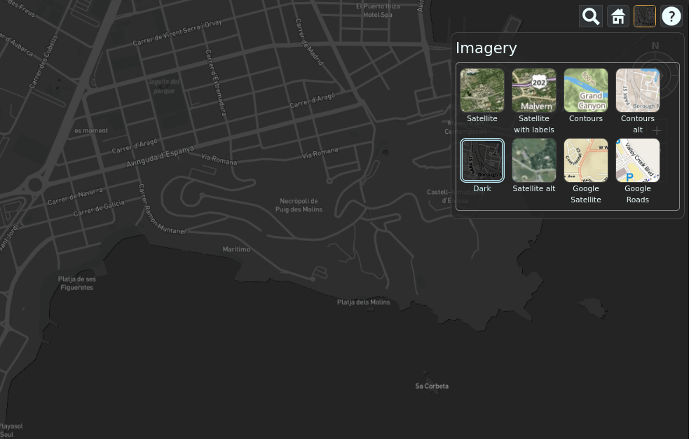
The Imagery tool lets you change the mapping/imagery style.
The Imagery choices offered include satellite imagery, street mapping and high contrast ‘dark’ layers for use with colourful overlays.
To choose the desired imagery:
Click on the Imagery
icon.The Imagery dialog box will appear and the various imagery options will be displayed.

Choose the desired Imagery.
The same will be reflected on the map.
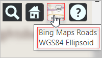
The Imagery icon and the mouse-over text will be changed depending upon the selected imagery.
For Example: On selecting the Bing Maps Road imagery, the following icon and mouse-over text will be displayed.
You can also enable/disable the underlying 3D terrain here.
By default, the 3D terrain is disabled to improve performance.
You can enable it by clicking the Toggle 3D Terrain
 icon located at the bottom-left of the interface.
The same will be reflected on the map.
 Navigation Instructions
The Navigation Instructions tool will display the navigation instructions for using the 3D interface on your computer and mobile.
Click on Navigation Instructions
icon.The Navigation Instructions dialog box will appear.
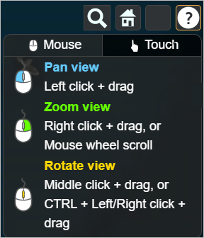
For navigating the 3D Interface on your computer, click on the Mouse
 tab.
tab.For navigating the 3D Interface on your mobile, click on the Touch
 tab.
tab.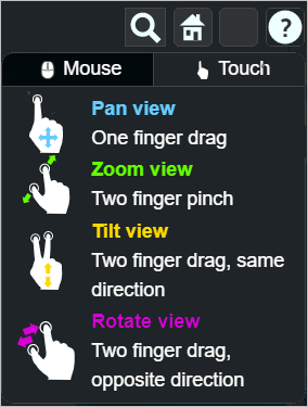
 Full Screen View
To enable the Fullscreen view:
Click on
icon located at the bottom right of the 3D Interface.
To exit the Fullscreen view:
Click on
 icon located at the bottom right of the 3D Interface.
Hiding Layers
Any created Layer(s) will be displayed on the map and the corresponding checkbox(es) will be displayed in a box which is located on the right side of the interface.
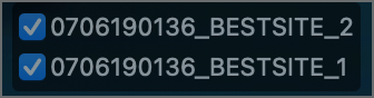
You may enable or disable the layers as per your requirement by simply checking and unchecking the checkboxes.
Map Management Menu Elements

The map tools located at the bottom of the interface lets you manage several elements which is detailed in the following section.
The left side of the bottom of the interface contains a number of tools which can be used to improve the interactivity of the interface.
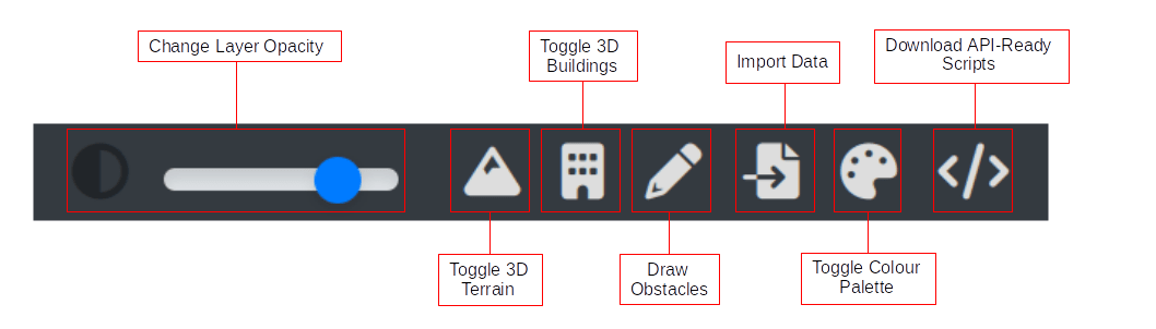
The right side of the bottom of the interface contains the decimal degrees location of the current transmitter location. This is a duplication of the information which is already available in the menu on the left of the interface, and is provided as a quick reference.
Changing Layer Opacity
You can change the opacity of the layer(s) on the map with the help of the opacity slider.

To increase the opacity, move the slider to the right.
To reduce the opacity, move the slider to the left.
Toggle 3D Terrain
You can toggle (enable/disable) the 3D Terrain as per your requirements by clicking on the Toggle 3D Terrain icon. For performance, 3D terrain is disabled by default.
- icon indicates that the 3D Terrain has been disabled.
 icon indicates that the 3D Terrain has been enabled.
Please note that when you enabled 3D buildings, 3D terrain will automatically be enabled.
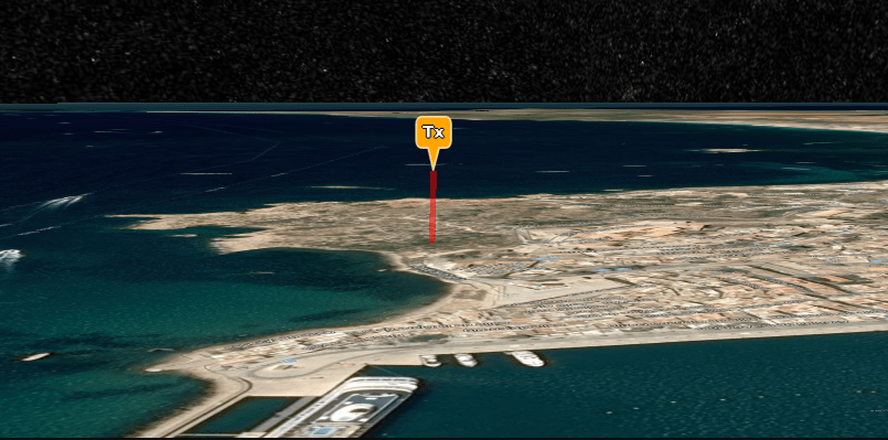
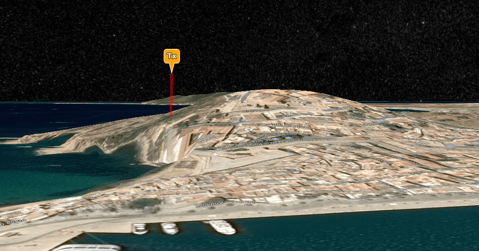
Following are the screenshots for reference showing the changes in the Map when the 3D Terrain is disabled and enabled:
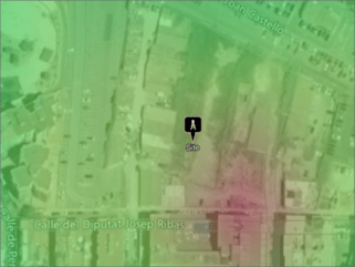
Map when the 3D Terrain is Disabled
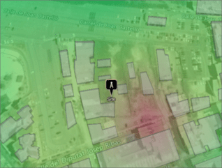
Map when the 3D Terrain is Enabled
 Toggle 3D Buildings
You can toggle (enable/disable) the 3D Buildings as per your requirement by clicking on the Toggle 3D Buildings icon. For performance, 3D buildings area disabled by default.
- icon indicates that the 3D Buildings have been disabled.
 icon indicates that the 3D Buildings have been enabled.
Please note that when you enabled 3D buildings, 3D terrain will automatically be enabled.
Following are the screenshots for reference showing the changes in the map when the 3D Buildings are disabled and enabled:
Map when the 3D Buildings are Disabled
Map when the 3D Buildings are Enabled
 Draw Custom Clutter
The “Draw Obstacles” tool is used for drawing your own custom clutter, with support for polygons. Please consult the clutter reference for more information.
 Import Data
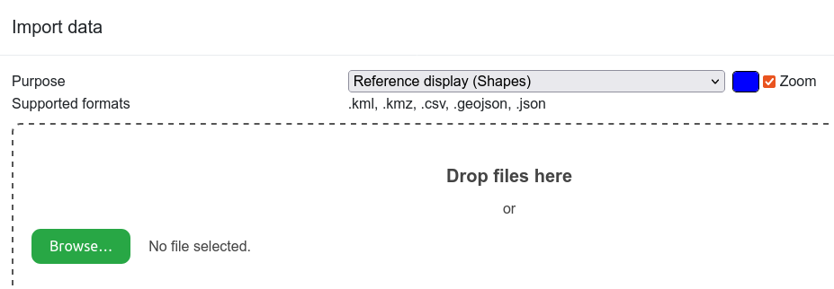
You can import structured data in different open formats by clicking on the . This will open a dialog modal window.
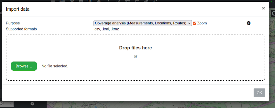
This modal window is separated into the following sections:
Purpose - This is the purpose for your reference data and will determine how your data is handled and which tool may be used eg. Best Site Analysis.
Zoom - When this is selected, after a successful import of your reference data it will move your viewer to your data location.
Supported formats - This will show you the supported format of file based on your selected “Purpose”. Please note that different purposes require different formats.
File drop area or Select file to upload - This is the location where you add your file. You can either drag-and-drop your file over the area, or you can use the button to locate the file on your system.
Help - The help button in the top right is used to provide additional information about the utilities to aid you in understanding how to work.
To make use of this tool simply select your chosen “Purpose” and upload your data in one of the specified formats.
At any point if you wish to remove your reference data from the map then you can simply click on the “Clear Layers”  button along the top of the interface.
File Validation
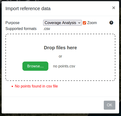
Regardless of the “Purpose” selected, your files will be validated when you upload them. This ensures that your files will work with the interface and be interpreted correctly.
If you have an error in your reference data then this will be displayed in the modal window.
Reference Display (Shapes on the map)
If you select “Reference Display” from the “Purpose” dropdown then this can be used to display imported data on the map such as polygons or pins.
When you select this option from the “Purpose” dropdown this will also show a new colour picker input which can be used to set the colour of your import data when it is drawn on the map.
This functionality can be used to create guides on the map where you can visualise where certain points or boundaries may be. For example, you may upload a CSV of points to indicate important landmarks, or you may upload a GeoJSON file which includes a boundary.
Below shows uploaded points using the “Reference Display” from a CSV:
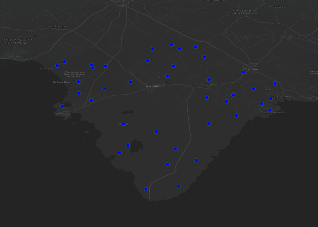
Below shows a sample CSV which was partially used to produce the above screenshot:
longitude,latitude,rssi
3.0505242,39.2707224,-70
3.0807366,39.2866678,-50
3.0560174,39.304735,-92
3.068377,39.2935764,-90
3.0340447,39.3100479,-67
3.0910363,39.3100479,-75
3.0381646,39.295702,-81
3.0632271,39.2842762,-91
Below shows a boundary uploaded using the “Reference Display” from a GeoJSON file:
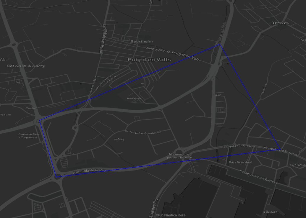
Below shows the GeoJSON which was used to produce the above screenshot:
{
  "type": "FeatureCollection",
  "features": [
    {
      "type": "Feature",
      "properties": {},
      "geometry": {
        "coordinates": [
          [
            [
              1.4256018139448656,
              38.92015233473046
            ],
            [
              1.4280509904125438,
              38.91581165124461
            ],
            [
              1.4449950785628118,
              38.91780215762395
            ],
            [
              1.441954782658172,
              38.92844609186906
            ],
            [
              1.4256018139448656,
              38.92015233473046
            ]
          ]
        ],
        "type": "Polygon"
      }
    }
  ]
}
Coverage Analysis (Measurements | Properties)
If you select “Coverage Analysis” from the “Purpose” dropdown then this powerfule utility can be used for several purposes:
Upload location data eg. zip / postal codes which can be used to gather metrics about coverage for areas and points.
Upload RF survey data which can be used to calibrate and optimise simulation settings by reporting the error
Importing Locations
You can upload a CSV with data about multiple points, for example customer properties by ZIP or UPRN.
For basic ‘points’ your CSV should follow the following rules:
The following fields are accepted:
idis a unique identifier of the point.latitudeis the latitude coordinate of the point. Should be a decimal value between -180 and 180.longitudeis the longitude coordinate of the point. Should be a decimal value between -90 and 90.groupis an optional field which allows you to group certain points together.
Your CSV must contain a header indicating the ordering of your fields.
An example CSV might look something like the below:
id,longitude,latitude,group
Point 1,3.0505242,39.2707224,SOUTH DISTRICT
Point 2,3.0807366,39.2866678,SOUTH DISTRICT
Point 3,3.0520286,39.3742523,NORTH DISTRICT
Point 4,3.0678215,39.3787639,NORTH DISTRICT
After successfully uploading your CSV it will be parsed and the interface will automatically draw your points onto the map.
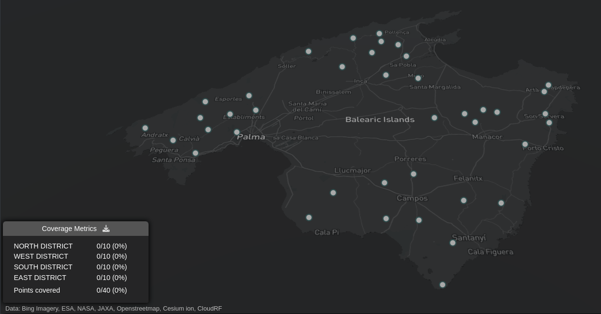
You may notice that a new window will be added to the bottom left of the screen. This is a live-updating metrics report which gives you details about your calculations, giving indications as to whether your points are covered or not.
If you next click on the map and run through a calculation you should see the points being coloured based on the signal strength but also the metrics report should update automatically when new calculations cover points.
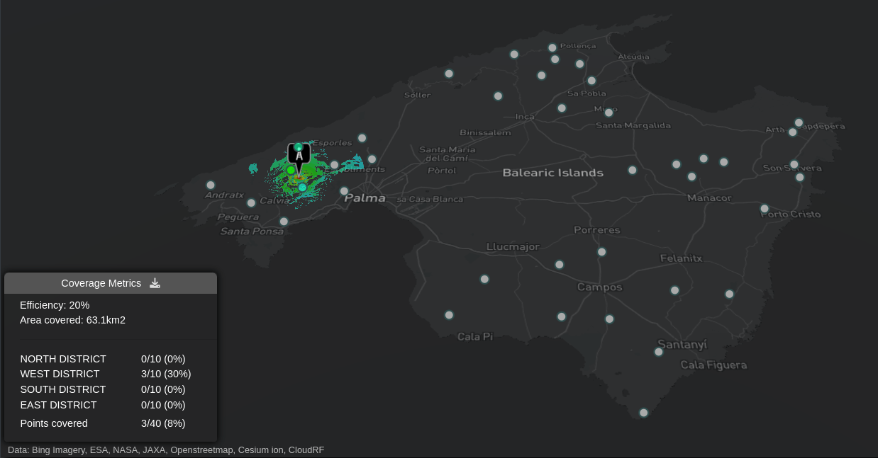
As you add new calculations this will update the metrics report showing you how much coverage you have in total. Each group as defined in your CSV will also be calculated based on its coverage.
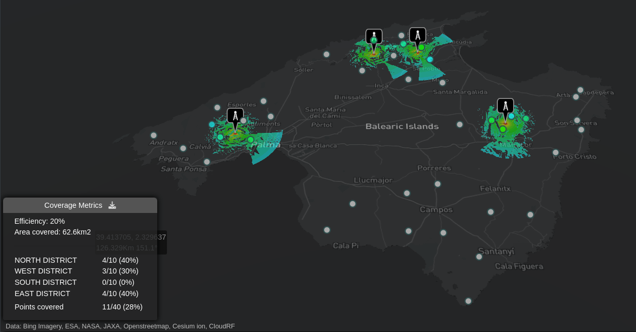
As you do multiple calculations this will build up your available layers on the map. As you check/uncheck them it will automatically update your metrics report in the bottom left of the interface. This is useful for seeing the effect removing a single layer has on an overall network.
In the “Coverage Metrics” window you can click on the “Download Coverage Metrics Report” icon  to obtain a report from your calculations. This is a
 txt file with information:
Location Coverage Metrics Report
Thu Apr 06 2023 12:56:54 GMT+0100 (British Summer Time)
Cloud-RF

NORTH DISTRICT: 4/10 (40%)
WEST DISTRICT: 3/10 (30%)
SOUTH DISTRICT: 2/10 (20%)
EAST DISTRICT: 4/10 (40%)

TOTAL COVERAGE: 13/40 (33%)

Layers:
0406125414_My_Site
0406125639_My_Site
0406125642_My_Site
0406125645_My_Site
0406125651_My_Site
Import Survey Data
You can upload a CSV with field measurements for easy modelling calibration. This was developed with CSV output from Cellmapper which is recommended for cellular surveys.
For basic ‘measurements’ your CSV should follow the following rules:
The following fields are accepted:
latitudeis the latitude coordinate of the point. Should be a decimal value between -180 and 180.longitudeis the longitude coordinate of the point. Should be a decimal value between -90 and 90.rssiis the measured signal strength in dBm. For cellular this needs to be received power not RSRP etc
Your CSV must contain a header indicating the ordering of your fields.
An example CSV might look something like the below:
longitude,latitude,rssi
3.0505242,39.2707224,-77
3.0807366,39.2866678,-82
3.0520286,39.3742523,-83
3.0678215,39.3787639,-88
Your CSV will be automatically validated when you upload it, if there are any errors then this will be displayed in the dialog window.
After successfully uploading your CSV it will be parsed and the interface will automatically draw your points onto the map and compute the delta between any visible layer upon it.
You may notice that a new window will be added to the bottom left of the screen. This is a live-updating metrics report which gives you details about the computed error. A good error value is less than 6dB. Anything greater than 9dB requires adjustments to your modelling parameters.
If you next click on the map and run through a calculation you should see the points being coloured based on the signal strength but also the metrics report should update automatically where new calculations cover points.
As you do multiple calculations this will build up your available layers on the map. As you check/uncheck them it will automatically update your metrics report. This is useful for comparing settings.
MANET Tool (A list of network nodes)
If you select “MANET Tool” from the “Purpose” dropdown then this can be used to import points for use with the MANET tool (GPU required). This is useful when you wish to use the MANET tool but don’t want to have to keep redrawing markers at the same locations if you want to test different profiles for example.
Please note that when you upload your file using “MANET Tool”, each point in your uploaded file will be applied with the same values that you currently have set for your settings.
After you submit your uploaded file a MANET calculation will be fired off immediately using your settings and preferences.
Below shows the result of a MANET calculation after being uploaded from a KML file:
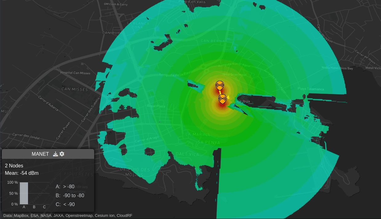
The above screenshot is taken from the following KML:
<?xml version="1.0" encoding="UTF-8"?>
<kml xmlns="http://www.opengis.net/kml/2.2">
  <Document>
    <Placemark>
      <name>Point 1</name>
      <Point>
        <coordinates>
          1.4397022,38.9146682,0
        </coordinates>
      </Point>
    </Placemark>
    <Placemark>
      <name>Point 2</name>
      <Point>
        <coordinates>
          1.440185,38.9130821,0
        </coordinates>
      </Point>
    </Placemark>
  </Document>
</kml>
For more information please consult the section relating to the MANET planning tool.
Best Site Analysis (An area for analysis)
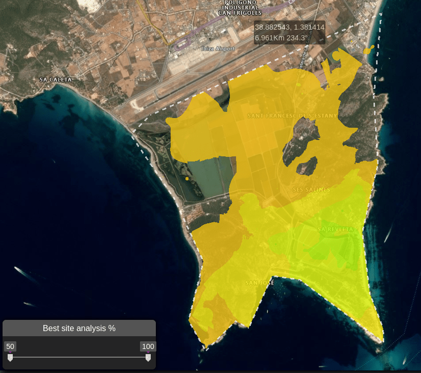
If you select “Best Site Analysis” from the “Purpose” dropdown then this is used to upload a polygon of a boundary which is used with the best site analysis functionality. This is useful if you are working with very specific boundaries and don’t wish to keep redrawing the area. Instead you can upload your file and have the calculation repeated with the same values every time.
Upon successful upload of your boundary the best site analysis tool will be immediately fired off using your current settings.
For more information please consult the section relating to the best site analysis planning tool.
Automatic processing (Process a spreadsheet)
If you select “Automatic processing” from the “Purpose” dropdown then this will enable you to upload a simple CSV spreadsheet describing the sites in your network. This uses a subset of what is available in the API and all other settings will be set in your form at the point of upload eg. Radius and Resolution.
This is a simplified way to use the API via the user interface which has limited options compared to the full examples documented on GitHub
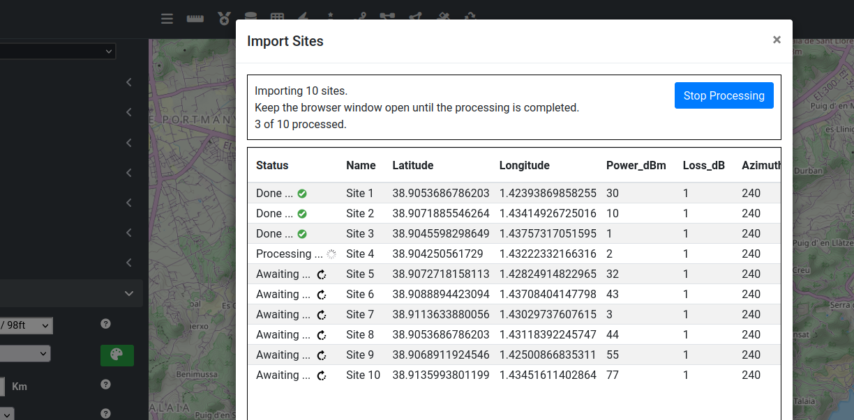
The CSV format must conform to one of two standards; a short format or a long format.
Short format CSV
Your CSV files must have these column headers:
“Name”
“Latitude”: between -90 and 90 (required)
“Longitude”: between -180 and 180 (required)
“Power_dBm”: (required)
“Loss_dB”
“Azimuth_deg”: between 0 and 359
“Downtilt_deg”: between 0 and 359
“Height_m”: between 0.1 and 60000 (required)
“Gain_dB”
Example CSV
Name,Latitude,Longitude,Power_dBm,Azimuth_deg,Downtilt_deg,Height_m,Gain_dB,Loss_dB
Site 1,38.9053686786203,1.42393869858255,30,240,10,6,8,1
Site 2,38.9071885546264,1.43414926725016,10,240,10,1,8,1
Site 3,38.9045598298649,1.43757317051595,1,240,10,10,8,1
Site 4,38.904250561729,1.43222332166316,2,240,10,11,8,1
Site 5,38.9072718158113,1.42824914822965,32,240,10,10,8,1
Site 6,38.9088894423094,1.43708404147798,43,240,10,9,8,1
Site 7,38.9113633880056,1.43029737607615,3,240,10,7,8,1
Site 8,38.9053686786203,1.43118392245747,44,240,10,8,8,1
Site 9,38.9068911924546,1.42500866835311,55,240,10,9,8,1
Site 10,38.9135993801199,1.43451611402864,77,240,10,7,8,1
Long format CSV
Your CSV files must have these column headers:
“Site”
“Latitude”: between -90 and 90 (required)
“Longitude”: between -180 and 180 (required)
“Height_m” (required)
“Frequency_MHz”: between 2 and 100000(required)
“Bandwidth_MHz”: between 0.1 and 200
“Power_W” (required)
“Receiver_Height_m”: between 0 and 60000
“Receiver_Gain_dBi”: between -30 and 60
“Receiver_Sensitivity_dBm”
“Antenna_Pattern”: Pattern name or “Custom”
“Antenna_Polarisation”: “V” for vertical or “H” for horizontal
“Antenna_Gain_dBi”
“Antenna_Loss_dB”
“Antenna_Azimuth_deg”: between 0 and 359
“Antenna_Tilt_deg”: between 0 and 359
“Antenna_Horizontal_Beamwidth_deg”: between 0 and 360 (required for custom patterns)
“Antenna_Vertical_Beamwidth_deg”: between 0 and 360 (required for custom patterns)
“Front_to_back”: between 0 and 360 (required for custom patterns)
“Noise_floor_dBm”
“Measured_units”
“Colour_schema”
“Model”
“Context”
“Diffraction”
“Reliability”
“Profile”
Example CSV
Site,Latitude,Longitude,Height_m,Frequency_MHz,Bandwidth_MHz,Power_W,Antenna_Pattern,Antenna_Polarisation,Antenna_Loss_dB,Antenna_Azimuth_deg,Antenna_Tilt_deg,Antenna_Gain_dBi,Noise_floor_dBm,Model
Site 1,38.9053686786203,1.42393869858255,10,446,1.4,30,OEM Half-Wave Dipole,V,0,240,10,8,-120,Egli VHF/UHF (< 1.5GHz)
Site 2,38.9071885546264,1.43414926725016,11,800,10,10,OEM Half-Wave Dipole,V,10,240,10,8,-90,Egli VHF/UHF (< 1.5GHz)
Site 3,38.9045598298649,1.43757317051595,20,2400,20,1,OEM Half-Wave Dipole,H,11,240,10,8,-70,Egli VHF/UHF (< 1.5GHz)
Site 4,38.904250561729,1.43222332166316,15,2100,22,2,OEM Half-Wave Dipole,V,4,240,10,8,-180,Egli VHF/UHF (< 1.5GHz)
Site 5,38.9072718158113,1.42824914822965,7,900,1.9,32,OEM Half-Wave Dipole,H,5,240,10,8,-90,Egli VHF/UHF (< 1.5GHz)
Site 6,38.9088894423094,1.43708404147798,30,1700,1.8,43,OEM Half-Wave Dipole,V,6,240,10,8,-120,Egli VHF/UHF (< 1.5GHz)
Site 7,38.9113633880056,1.43029737607615,31,1800,18,3,OEM Half-Wave Dipole,H,1,240,10,8,-140,Egli VHF/UHF (< 1.5GHz)
 Toggle Colour Palette
At the bottom of the interface there is a palette icon . When you click on this button this will hide your colour palette on the right side of the screen. This can be useful when you are working on devices with smaller screen sizes as the colour palette may obscure certain interface elements.
 Download API Ready Scripts
If you wish to build up a number of settings which you can then take away and use in your own scripts which make use of the Cloud-RF public API, then you can click on the “Download API ready scripts” icon.
When you click on this icon you will be presented with a modal window:
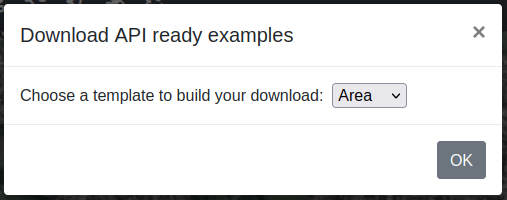
From the dropdown you can select one of the following endpoints:
Area will download scripts with your current settings suitable for an
areacalculation.Path will download scripts with your current settings suitable for a
pathcalculation.Points will download scripts with your current settings suitable for a
pointscalculation.
Regardless of which you choose, each will download a respective ZIP file with a number of files which have been built with your specific settings. The files included should contain the following:
readme.txtwith some basic instructions on hbow to use the downloaded scripts.sites.csvwith your transmitter and, if present, receiver locations along with their network names.template.jsonwith a raw request as it would be made to your chosen endpoint.A Python script named after the chosen endpoint, such as
area.pyif you selected Area.cloudrf.iniwith some configuration values based on your particular values, such as your API key, and the URL for the Cloud-RF public API.cloudrf.pyis the Python base class if you wanted to extend your own requests and is based on the Python script available on GitHub.
My obstacles
Custom obstacles or Clutter can be defined as anything which could impede a signal’s path.
For RF planning purposes, the clutter can predominantly be trees and buildings. As the trees and the buildings vary greatly in density, we have included their different types.
The global clutter data for telecommunications planning is very expensive, and often outdated, despite their price. We have developed a much more flexible way of self-generating accurate clutter models.
Whether you need to define one big building which is being planned for construction or you need to upload a plan for an entire city - we support both DIY (Do It Yourself) and BYO (Bring Your Own) clutter.
DIY Clutter - You can draw your own clutter directly in the Cloud-RF interface to meet your requirements, defining the Type of the clutter.
BYO Clutter - You can upload your own KML / GeoJSON file directly.
DIY Clutter
DIY clutter allows you to draw and build your clutter directly in the Cloud-RF interface to meet your requirements.
Click on the Draw obstacles button
icon to draw custom clutter located at the bottom-left of the interface.The Custom Clutter Dialog box will appear.
For information regarding Drawing Clutter, refer to the Drawing a Polygon section.
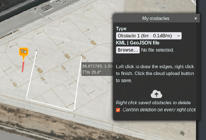
The dialog box is split into several parts.
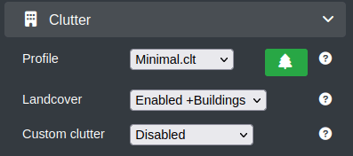
Type determines the type of the material under which you clutter will be allocated. This is for DIY clutter. The value set here will be taken based upon your clutter profile which you select in the “Clutter” menu from the “Profile” dropdown on the input menu on the left of the interface. This is used to determine the height and attenuation of the clutter.
The “Browse”/”File” button is used to submit KML or GeoJSON files for BYO clutter.
The upload button is used to send your clutter to the Cloud-RF service to handle your clutter.

The checkbox at the bottom for “Confirm deletion on every right click” is a safety catch as you may have multiple clutter on your profile - rather than having to confirm deletion of every one you might decide to disable this checkbox at which point right-clicking on a clutter will instantly delete it without any confirmation.
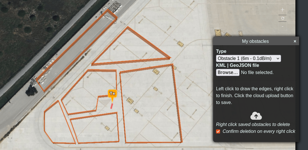
Drawing Custom Clutter
To define a clutter polygon:
Click on the Draw Obstacles
icon located at the bottom-left of the interface.Left-Click on the map to draw the edges of the polygon as per your requirement.
Right-Click to finish. You can repeat as many times as necessary to draw multiple polygons with the same properties.
The Custom Clutter Dialog box will also be displayed.
For more information, refer to the Custom Clutter section.
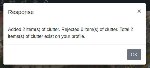
After you have finished drawing your polyline clutter you should then click on the upload button.
You will be presented with an overview of the clutter which was uploaded to your profile.
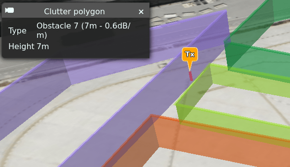
When you close the clutter menu your drawn polyline will be displayed on the map. You can left-click on it to show its properties.
Selecting/Changing Clutter Type and Height
Clutter properties are applied based on the Type you choose from the clutter dialog box.
The attenuation and height for these types are defined in your clutter profile which is selected from the “Environment” menu.
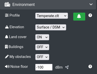
You can choose different clutter profiles to match your environment, or you can create your own clutter profile to define your height and attenuation by clicking on the “Clutter Manager” button. 
From the clutter profile manager you can create and define your own attenuation and heights for listed materials.
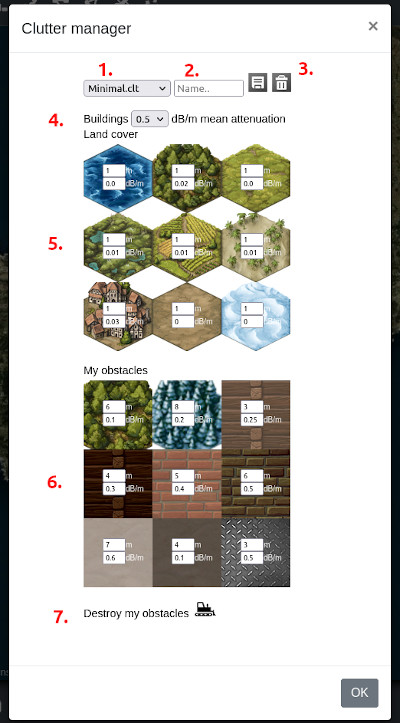
Selected Profile
Save new profile as name
Save and delete name listed in 2.
Building attenuation
Land cover types
My obstacle (clutter) types
Delete my obstacles
Deleting Clutter Profile
If you wish to delete a custom clutter profile then please enter its name into the input box then press on the delete button. Please note that the name must exactly match, including the casing and the extension name. You are also unable to remove system clutter profiles.
BYO Clutter
Uploading a KML / GeoJSON file
This is a BYO type of clutter.
You can import multiple clutter items as a KML or GeoJSON file.
Open the custom clutter menu by selecting the Draw obstacles button
icon located at the bottom-left of the interface.Click on Choose File button.
Select the desired KML/GeoJSON file.
Click on the Upload
icon to save the clutter.A Response box will be displayed stating that the Clutter has been added.
Viewing the Defined Clutter
After drawing, defining and uploading the clutter, you can view the defined clutter on the map.
Polygon Clutter
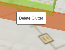
Deleting Clutter
To delete a clutter:
Right-Click on the respective clutter on the map.
If you had the “Confirm deletion on every right click” checked in the custom clutter dialog box then you will be prompted to confirm deletion of each peice of clutter. Otherwise the clutter will be deleted without any confirmation.
You can also delete all clutter in your profile by opening the clutter manager and pressing the “Delete my obstacles” button.
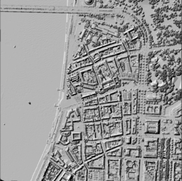
LiDAR
LiDAR data is the highest accuracy data available and is available for many cities at 2m resolution.
Check the coverage map to see if you are covered.
It’s a surface raster, hence, it is not permeable like the custom clutter but is very useful for line of sight analysis as even trees and bushes are represented.
Mobile View
Touch Screen Gestures
You can pan view, zoom, tilt and rotate on your touch screen phone using the following finger gestures:
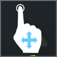
Pan Map
You can pan the map by selecting with a single finger and dragging your finger across the screen.
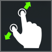
Zoom Map
You can zoon the map by placing two fingers on the map and pinching the fingers together or away from one another to either zoom in or zoom out, respectively.
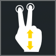
Tilt Map
You can tilt the map by placing two fingers on the map and dragging them both in the same direction up or down the screen.
Rotate Map
You can rotate the map by placing two fingers on the map and rotating your hand clockwise or counter-clockwise.

Outputs
Embed Code
The new Embed Code functionality lets you Copy the HTML code and upload it to your website with the desired filename and the html extension.
You can reap the following benefits and more using the HTML Embed Code functionality:
Build your own Coverage Map.
Create radio heatmap for your website.
Add Google Maps to your website.
Add RF Coverage on the Google Maps.
For more information regarding this, refer to the Embed Code Benefits topic.
To access the Embed Code functionality:
Click on My Archive
 button on the Function Menu.
The My Archive dialog box will appear.
Click on the HTML Embed Code
 icon.
icon.The Embed Code dialog box will appear.
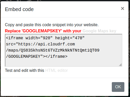
You can copy the HTML code snippet from here and paste it to your website.
Replace the
GOOGLEMAPSKEYin the code with your Google Maps Key.You may Test and Edit the code snippet with the help of HTML editor
Build Your Own Coverage Map
Are you a wireless internet service provider or an organisation that requires an online coverage map to be displayed on their website?
Building your own Coverage Map is just a few clicks away…
The most basic option is to accomplish this is using an arbitrary polygon on a free map like Google Maps. However, if you require a beautiful and accurate physics-based coverage map, at no extra cost, CloudRF’s Embed Code functionality is all you need.
Using the CloudRF’s Embed Code functionality is the easiest way to add a map to your website or blog that supports the HTML content. You just need to copy-paste an HTML code snippet to your website and replace the GOOGLEMAPSKEY in the code with your own Google Maps API key.
For further information regarding Hosting your own Network Map, click on this link.
Create Radio Heatmap for Website
The Embed Code functionality lets you create the radio heatmap for your website.
With the help of GIS mapping and the LIDAR Imaging from the satellites, the CloudRF tool will output a heatmap of the signal strength on the 3D map. Hence, you can create the radio heatmap for your website and also determine how well your signal propagate based on some variables that you configure in the tool.
For further information, refer to this link.
Add Google Maps to the Website
All you need is a web browser and you are just three steps away from adding the Google Map plus RF layer to your website: