The trouble with radio planning software
Radio planning software has a patchy reputation. Regardless of cost, the criticism, especially from novice users, is generally that results “do not match the real world”. The accuracy of modelling software can be improved with training, better data, tuned clutter etc but if you do not plan for the local spectrum noise, it will be inaccurate.
The reason modelling does not match the real world, is the real world is noisy, and noise is everything in digital communications. Spectrum noise will limit your network’s coverage and equipment’s capabilities. A radio that should work miles can be reduced to working several feet only when the noise floor is high enough.
Anyone expecting simulation software to produce an accurate result without offering an accurate noise figure will be forever disappointed as software cannot predict what the noise floor is in a given location at a given moment – you need hardware for that…
Spectrum sensing radios
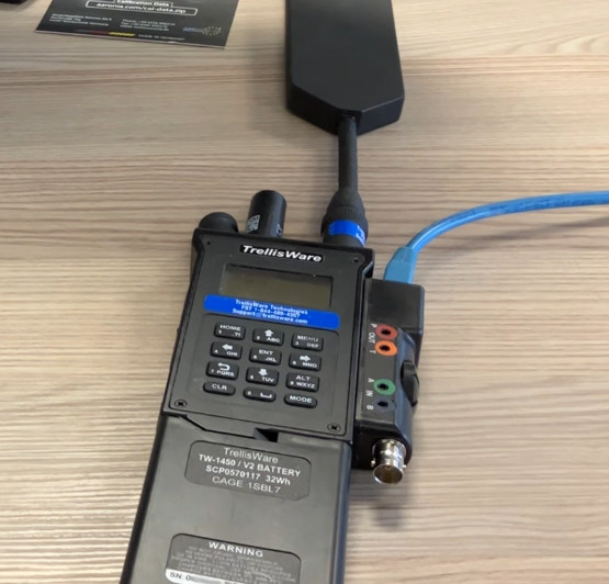
Modern software defined radios are capable of sensing the noise figure for the local environment. This allows operators, and cognitive radios, to make better choices for bands, power levels and wave-forms as narrow wave-forms perform better in noise than wider alternatives due to channel noise theory where noise increases with bandwidth.
For example, you can have a radio capable of 100Mb/s but it won’t deliver that speed at long range, at ground level, as it requires a generous signal-to-noise margin to function. This is why a speed demo is always at close range.
When spectrum data is exposed via an API, like in the Trellisware family of radios, it provides a rich source of spectrum intelligence which can be used for radio network management, and dynamic RF planning with third party applications. When we integrated this radio API last year, we were focused on acquiring radio locations, not spectrum noise. At the time we could only consider a universal noise floor value in our software so the same noise value was applied for all radios which was vulnerable to error as radios in a network will report different noise values.
Interference: a growing issue
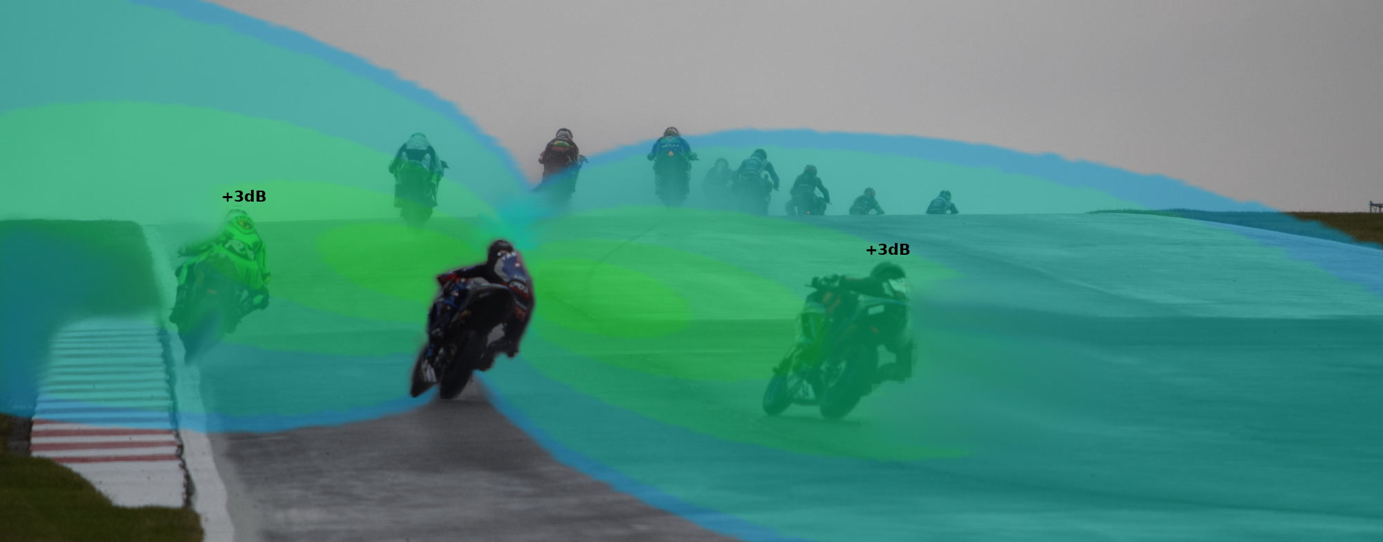
The single biggest communications problem we hear about, from across market sectors, is interference, either deliberate, accidental, or just ambient like in a city. The number of RF devices active in the spectrum, especially ISM and cellular bands, is increasing and in markets which were relatively “quiet”, such as agriculture. Some have always been problematic, such as motorsport, where the noise floor increases significantly on race days.
Spectrum management is a huge problem which won’t be fixed with management consultants or artificial intelligence. Regulators can, and are, restructuring spectrum for dynamic use but to use this finite resource efficiently, hardware and software vendors need to publish APIs and competing vendors need to be incentivised to work to common information standards.
As noise increases, the delta between low-noise RF planning results and real world results has the potential to grow. There’s anecdotal evidence that some private 5G network operators are experiencing so much urban noise they’ve given up on RF planning altogether, and have opted to take their chances using a wet finger and local knowledge. Skipping RF planning is a managed risk when a company has experienced staff (or they get paid for failure), but it does not scale and is a significant risk when working in a new area and/or with inexperienced staff.
A solution: The noise API
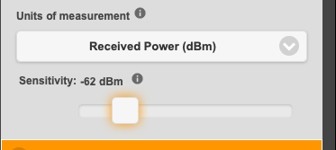
To address this challenge, we’ve developed a noise API to eliminate human error, and guesswork for noise floor values which has undermined the reputation of “low-noise” radio planning software.
Manual entry can now be substituted for a feed of recent, or live, spectrum intelligence to enable faster and more accurate network planning. Combined with our real-time GPU modelling, the API can model coverage for moving vehicles, with real noise figures.
There are two new API requests in v3.9 of our API; /noise/create; for adding noise, and /noise/get; for sampling noise. The planning radius is used as a search area so you can upload 1 or thousands of measurements, private to your account. The planning API will reference the data, if requested, and if recent (24 hours) local noise is available for the requested frequency, it will sample it and compensate for the proximity to the transmitter(s).
When no noise is available within the search radius, an appropriate thermal noise floor will be used based on the channel bandwidth and the Johnson-Nyquist formula. The capability can be used by our create APIs (Area, Path, Points, Multisite) by substituting the noise figure in the request eg. “-99” for the trigger word “database”.
{
  "site": "2sites",
  "network": "MULTISITE",
  "transmitters": [
    {
      "lat": 52.886259202681785,
      "lon": -0.08311549136814698,
      "alt": 2,
      "frq": 460,
      "txw": 2,
      "bwi": 1,
      "nf": "database",
      "ant": 0,
      "antenna": {
        "txg": 2.15,
        "txl": 0,
        "ant": 39,
        "azi": 0,
        "tlt": 0,
        "hbw": 1,
        "vbw": 1,
        "fbr": 2.15,
        "pol": "v"
      }
    },
    {
      "lat": 52.879223835785716,
      "lon": -0.06069882048039804,
      "alt": 2,
      "frq": 460,
      "txw": 2,
      "bwi": 1,
      "nf": "database",
      "ant": 0,
      "antenna": {
        "txg": 2.15,
        "txl": 0,
        "ant": 39,
        "azi": 0,
        "tlt": 0,
        "hbw": 1,
        "vbw": 1,
        "fbr": 2.15,
        "pol": "v"
      }
    }
  ],
  "receiver": {
    "alt": 2,
    "rxg": 2,
    "rxs": 10
  },
  "model": {
    "pm": 11,
    "pe": 2,
    "ked": 1,
    "rel": 80
  },
  "environment": {
    "clm": 0,
    "cll": 2,
    "clt": "SILVER.clt"
  },
  "output": {
    "units": "m",
    "col": "SILVER.dB",
    "out": 4,
    "res": 4,
    "rad": 3
  }
}:
In the example JSON request above, two adjacent UHF sites are in a single GPU accelerated multisite request. The sites both have a noise floor (nf) key with a value of “database”. Noise will be sampled separately for each site.
Demo 1: Motorsport radio network on race day
The local noise floor jumps ups significantly on race day compared with the rest of the time making planning tricky.
Demo 2: Importing survey data to model the “real” coverage across a county
By importing a spreadsheet of results into the API, we can generate results sensitive to each location.
A look forward to cognitive networks
Autonomous cognitive radio networks require lots of data to make decisions.
Currently, they can use empirical measurements of values such as noise to inform channel selection and power limits at a single node.
What they cannot do is hypothesise what the network might look like without actually reconfiguring. To do that requires a fast and mature RF planning API, integrated with live network data. Only then can you begin to ask the expansive questions like, which locations/antennas/channels are best for my network given the current noise or the really interesting future noise whereby the state now is known but the state in the future is anticipated.
As our GPU multisite API can model dozens of sites in a second, the future could be closer than you think…
References
API reference: https://cloudrf.com/documentation/developer/swagger-ui/
Hosted noise client: https://cloud-rf.github.io/CloudRF-API-clients/integrations/noise/noise_client.html
GPU multisite racetrack demo: https://cloud-rf.github.io/CloudRF-API-clients/slippy-maps/leaflet-multisite.html
 Jamming is a form of electronic attack which uses a stronger signal to disrupt target wireless devices.
DISCLAIMER: It is an offence to intentionally interfere with someone else’s use of the wireless spectrum in the UK.
The mention of its name also disrupts rational thinking amongst otherwise intelligent people and its common for spectrum planners and event managers to ignore signal theory when discussing its impact and revert to hollywood instead.
Originally used in warfare, it’s now commonly used in civil emergencies such as event protection, bomb disposal or hostage negotiation.
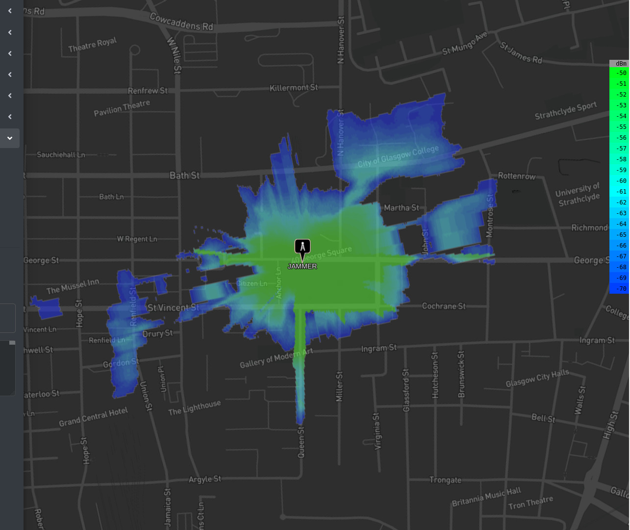
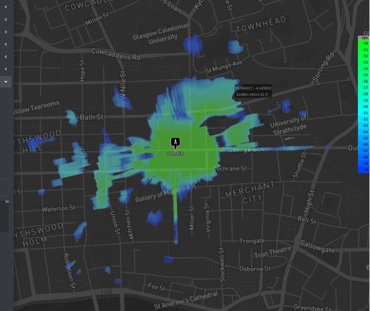
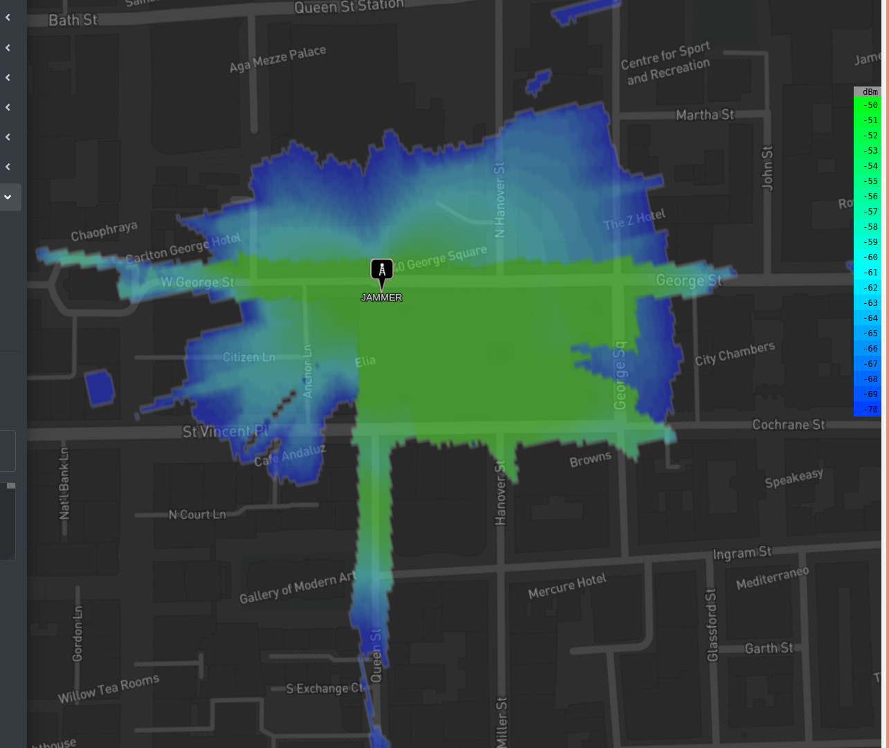
This blog uses modelling evidence to demonstrate the impact of jamming in a city and in the process, debunk popular jamming myths. The target band in all models is the 2.4GHz ISM band which is easily the busiest unlicensed band in the world and home to WiFi, Bluetooth, CCTV, Locks, Sensors, Drones and phones. The chosen location is George Square in Glasgow which is a large open surrounded by tall stone buildings. The antenna used is Omni-directional to visualise the effect in all directions.
Jamming is a form of electronic attack which uses a stronger signal to disrupt target wireless devices.
DISCLAIMER: It is an offence to intentionally interfere with someone else’s use of the wireless spectrum in the UK.
The mention of its name also disrupts rational thinking amongst otherwise intelligent people and its common for spectrum planners and event managers to ignore signal theory when discussing its impact and revert to hollywood instead.
Originally used in warfare, it’s now commonly used in civil emergencies such as event protection, bomb disposal or hostage negotiation.
This blog uses modelling evidence to demonstrate the impact of jamming in a city and in the process, debunk popular jamming myths. The target band in all models is the 2.4GHz ISM band which is easily the busiest unlicensed band in the world and home to WiFi, Bluetooth, CCTV, Locks, Sensors, Drones and phones. The chosen location is George Square in Glasgow which is a large open surrounded by tall stone buildings. The antenna used is Omni-directional to visualise the effect in all directions.