Enhancing accuracy with environment profiles

In radio planning, accurate terrain data is only half the story.

The other data you need, if you want accurate results, is everything above the surface such as buildings and trees.

This is known as land cover or in radio engineering; clutter data.

Clutter data

In October 2021, the European Space Agency released a global 10m land cover data set called WorldCover with 9 clutter bands.

In our opinion, the ESA data is a sharp improvement on a similar ESRI/Microsoft 10m land cover data set also published this year.

The land cover can be used to enhance coarse 30m data sets to distinguish between homes and gardens, or crops and rivers. It’s space mapped so has every recent substantial building unlike community building datasets which can be patchy outside of Europe.

This data was previously very expensive. A price reflected in the eye watering pricing of legacy Windows^TM planning tools.

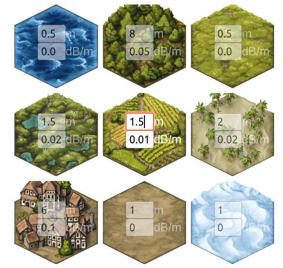
The data has 9 bands which have been mapped to 9 land cover codes in Cloud-RF^TM. Combined with our recent 9 custom clutter bands, we have 18 unique bands of clutter which you can use simultaneously.

Read more about the codes in the documentation here.

Explore the data we have on the ESA WorldCover viewer application here:

https://viewer.esa-worldcover.org/worldcover/

Custom clutter enrichment

We have integrated the 10m data into our SLEIPNIR^TM propagation engine which as of version 1.5, can work with third party and custom clutter tiles simultaneously, in different resolutions.

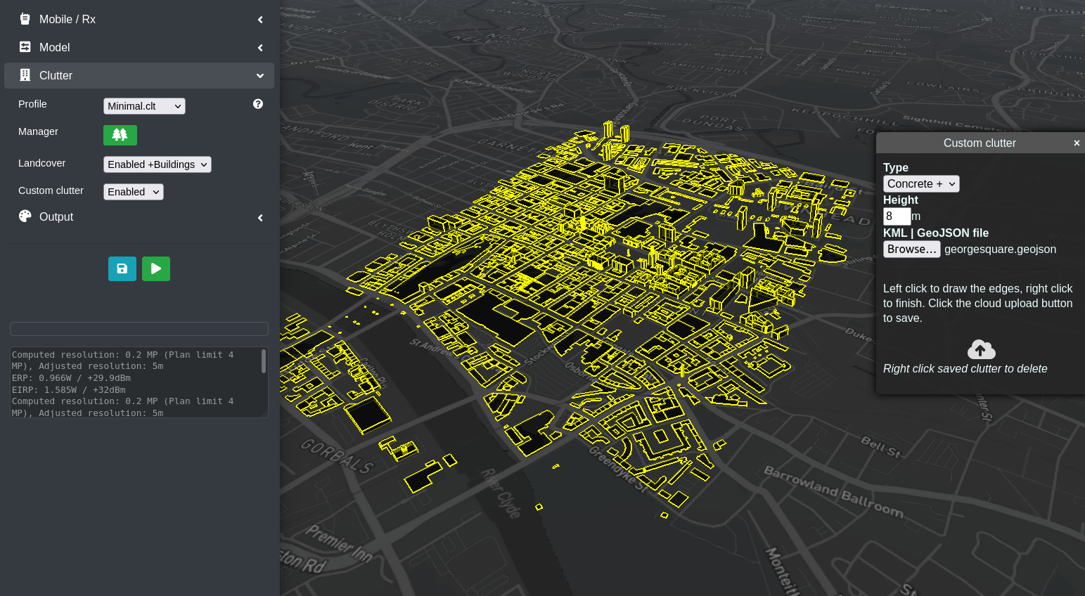
This is significant as it means you can have a 30m DSM base layer, enhanced with a 10m land cover layer, enriched further with a 2m building which you created yourself. Effectively this gives you a 10m global base accuracy with potential for 2m accuracy if you add custom obstacles. The interface will let you upload multiple items as a GeoJSON or KML file.

Demo 1 – The Jungle

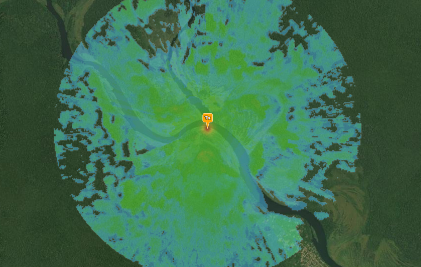
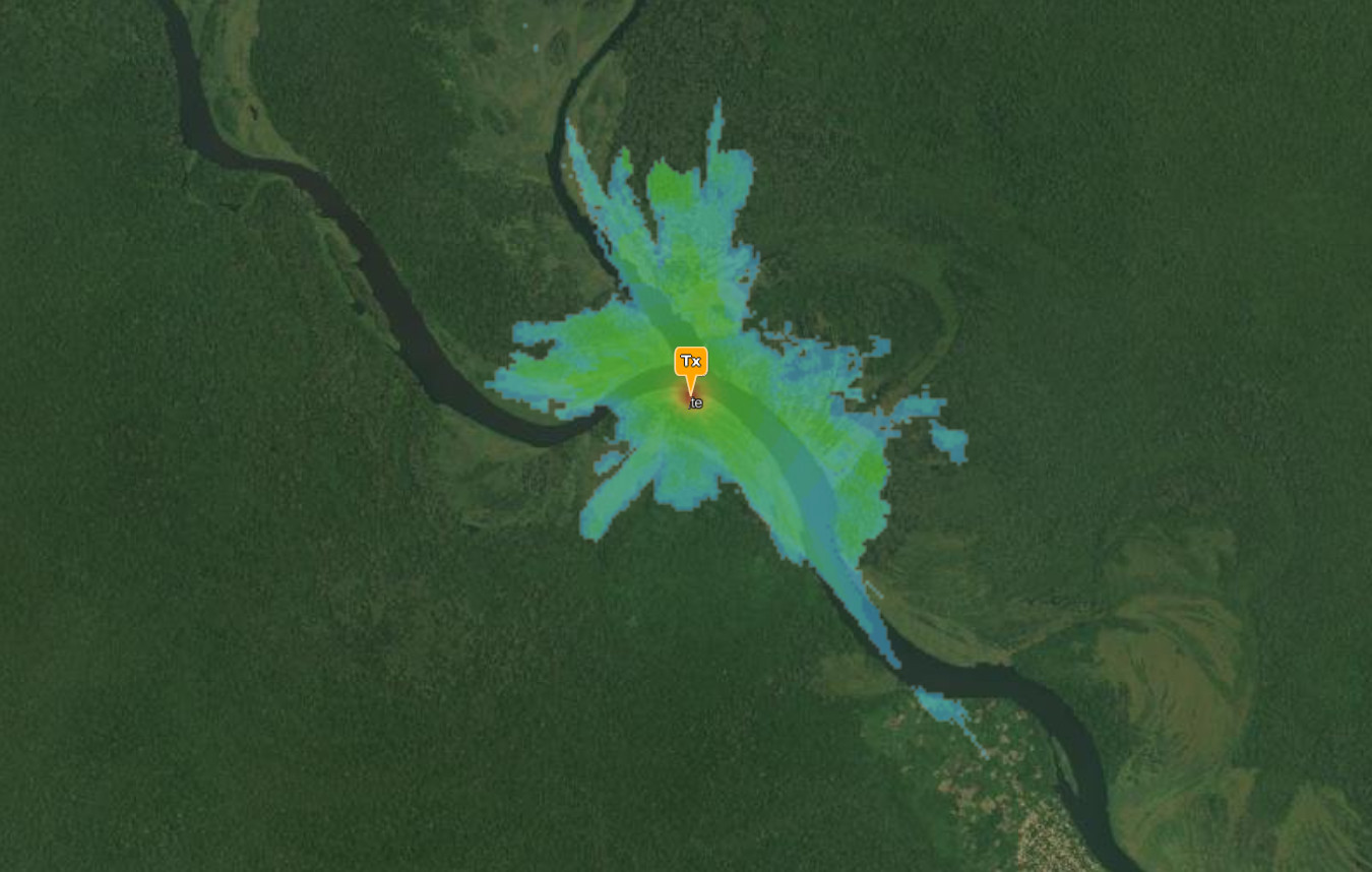
Always a tricky environment to communicate in, and model accurately due to dense tree canopies. In this demo, a remote region of the Congo has been selected at random for a portable VHF radio on 75MHz with a 3km planning radius.

This area has 30m DSM which out of the box produces an unrealistic plot resembling undulating flat terrain. This is because the thick tree canopy is represented as hard ground and the signal is diffracting along as if it were bare earth. The result therefore is that 3km is possible in all directions.

By adding our “Tropical.clt” clutter profile, calibrated for medium height, dense trees, we get a very different view which shows the effective range through the trees to be closer to 1km, or less, with much better coverage down the river basin, due to the lack of obstructions.

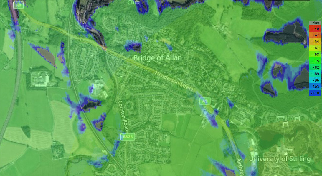
Demo 2 – A region without LiDAR

Scotland has very poor public LiDAR compared with England which has good coverage at 1m and 2m.

For this demo, Stirling was chosen which has 30m DSM only. A cell tower on a hill serving the town produces an optimistic view of coverage by default but when enhanced with a “Temperate.clt” clutter profile, calibrated for solid and tall town houses and pine forests (eg. > 50N, Northern Europe, Northern USA) we get a much more conservative prediction. As a bonus, the base resolution has improved three fold to 10m.

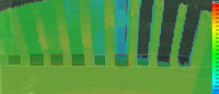
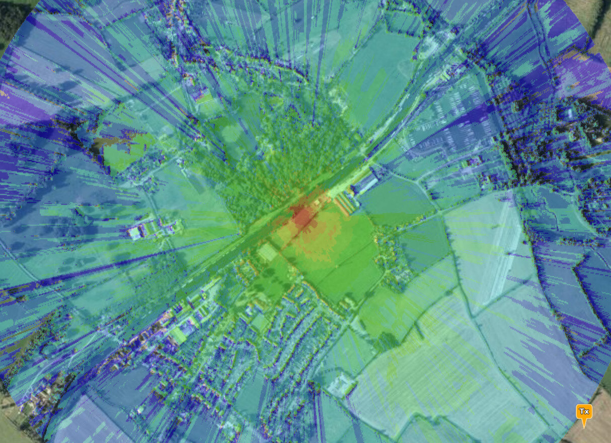
Demo 3 – A region with 2m LiDAR

You might think if you’ve got high resolution LiDAR data that’s enough. Wrong. Soft obstacles like trees especially will produce excessive diffraction as if they were spiky terrain. This manifests itself as optimistic ‘great’ coverage due to the diffraction coverage. By adding our “Temperate.clt” profile again we make trees absorb power and see where there are nulls in our coverage – beyond the houses and woods.

Despite our land cover being only 10m resolution, we are able to benefit from the full LiDAR resolution with 2m accuracy.

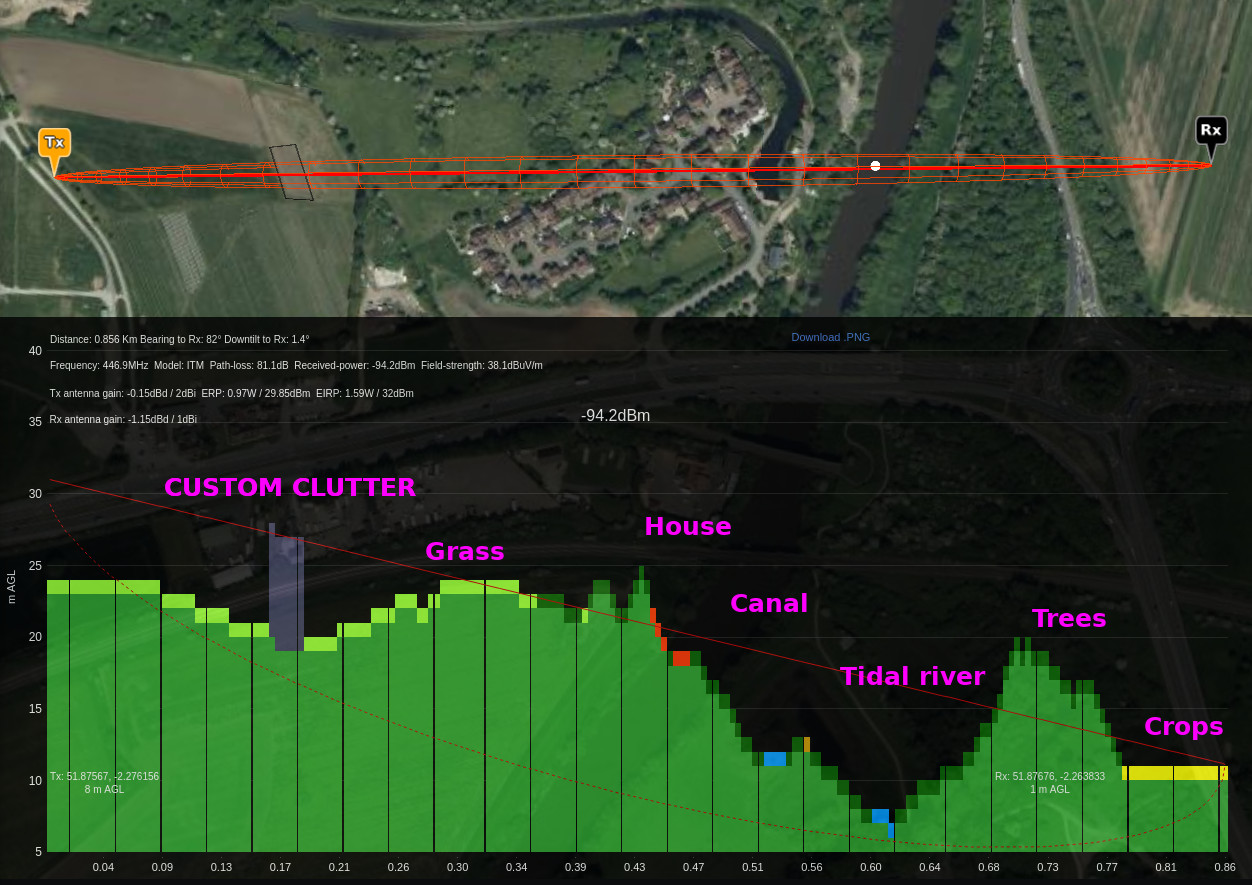
Inspecting a profile

The path profile tool will now show you colour coded land cover as well as custom clutter and 3D buildings. Crops are yellow, grass is green(!), Trees are dark green, built-up areas are red, 3D buildings are grey, water is blue…

The most significant feature in this image isn’t the coloured land cover, or the custom building (as both are features we’ve done before), or the fact we know the tidal river Severn sits lower than the man-made Canal beside it, It’s the fact that both are being used in the same model at the same time. They are different sources, different resolutions, different densities…

Path profile for 860m link showing 2m LiDAR, 10m Land cover and 2m custom building

Using and editing a profile

Once you’ve got the hang of switching profiles you may find it needs optimising for your region. With the clutter manager in the web interface, premium customers can create their own profile based on field measurements for highly accurate predictions. After all no two forests or neighbourhoods are the same density.

Create your perfect profile and save it to your account. The system has 5 regional profiles ready for all users and you can add your own.

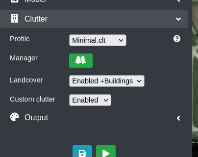
To use them, pick from the Clutter > Profile menu and ensure “Landcover” is set to “Enabled”.

If you have created custom clutter and want to use that, set Custom clutter to “Enabled” to blend it in.

For more see the web interface clutter section in the documentation.

Using clutter from the API

We played with a few designs before settling on this very simple template method where you set a profile within the environment menu as follows. This is a new value “clt” and you can still use the existing “cll” and “clm” values to manage the system clutter and custom clutter layers.

JSON request excerpt for a temperate “European” profile, with custom clutter, with 3D buildings and a 3D building density of 0.25dB/m

  "environment": {
        "clt": "Temperate.clt",
        "clm": 1,
        "cll": 2,
        "mat": 0.25
    },

Example for Jungle profile, without custom clutter, without 3D buildings.

  "environment": {
        "clt": "Jungle.clt",
        "clm": 0,
        "cll": 1,
        "mat": 0
    },

What’s next?

Now that we have highly configurable environment profiles. it’s time to tune them with field testing. We’ve bought a heap of comms equipment and will be using it to optimise these profiles with real world measurements.