We took a field trip to model LTE (4G) coverage in order to collect data we can use to develop calibration utilities and improve modelling as modelling is only as accurate as your inputs.
We focused on a single remote cell in the Peak District national park identified through cellmapper.net. We expected to find one cell only but were surprised to be serviced by several distant LTE cells, not evident in the crowd sourced app and equally significant, we established limited or no coverage in an area where a national map suggested coverage was available.
Key findings
- Data revealed the crowd-sourced coverage app was conservative in rural areas
- Data revealed the operator’s network map was optimistic in rural areas
- Modelling was matched with 2.5dB RMSE for a cell 12km away
- Modelling was on average accurate to 5.5 dB RMSE
- Improvements to modelling have been identified
Equipment and process
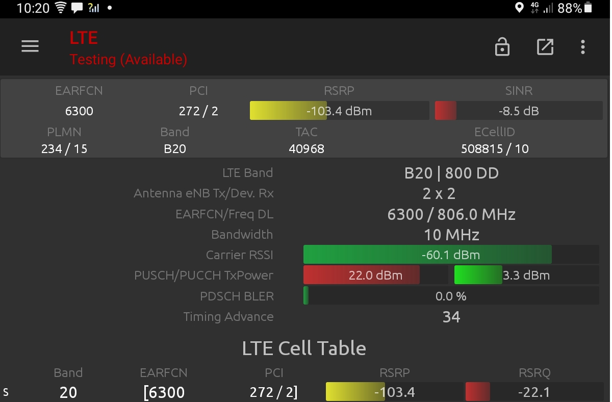
We used a rooted Samsung Galaxy Tab with an integrated Qualcomm X11 LTE modem, running both Network Signal Guru (NSG) and Cellmapper. NSG requires root access to lock to a cell which was necessary to prevent our survey tablet from hopping around not only protocols (2G,3G) but neighbouring cells.
Cellmapper is a crowd-sourcing app which writes signal strength readings to a CSV file, convenient for our analysis. Before embarking we planned a route around a remote cell on the edge of available coverage maps.
Both apps record various LTE power levels such as Received Power Received Signal (RSRP), Received Power Received Quality (RSRQ) and Received Signal Strength Indicator (RSSI). For this test we use RSSI which is typically a stronger value than the others as it is the measured carrier, irrespective of bandwidth.


Receiver measurement calibration
Radio receivers are subject to measurement error, typically in the range of 0.5 to 3.0dB for very expensive and consumer grade equipment respectively. As we were using a consumer grade Snapdragon 662 SoC with an X11 LTE modem, we needed to find out it’s measurement error. The Qualcomm datasheets we could find didn’t list this value so we used empirical measurements to establish it.
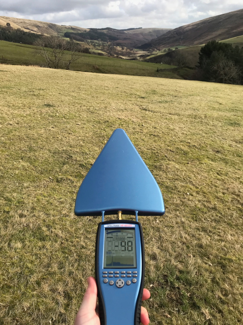
During our survey we paused at a site 3km from a tower with line of sight where we recorded continuous power readings with the tablet static on the ground for about 15 minutes. Consistency is essential for calibration. We have analysed these readings to establish a standard deviation in readings of 3.1dB for the X11 LTE modem, which puts it at the consumer end of the spectrum for survey device accuracy, in accordance with its price.
We use the error of 3.1dB in our analysis by subtracting it from the Root Mean Square Error (RMSE).
python3 receiver_calibration.py receiver_calibration_3km_LOS.csv
[-71.0, -71.0, -67.0, -71.0, -67.0, -69.0, -69.0, -69.0, -71.0, -77.0, -67.0, -71.0, -73.0, -71.0, -71.0, -71.0, -75.0, -69.0, -73.0, -69.0, -75.0, -69.0, -71.0, -79.0, -73.0, -65.0, -73.0, -71.0, -71.0, -75.0, -71.0, -73.0, -77.0, -75.0, -69.0, -75.0, -75.0, -73.0, -77.0, -73.0, -71.0, -75.0, -73.0, -79.0, -75.0, -71.0, -71.0, -75.0, -67.0, -73.0, -73.0]
Mean: -72.1dB
Error: 3.1dB
The survey
Setting off uphill from Derwent Dam car park with Sheffield’s man-of-the-mountain, Chris, we approached our target cell located on the hillside below us.
As we neared 500m we used NSG to lock onto a strong LTE signal which we believed was the target (CID 130256660, PCI 270), based on proximity and strength (-60dBm RSSI). It was in fact a tower on a distant hill 12 km to the south with line of sight, CID 131413770. Surprise number 1.
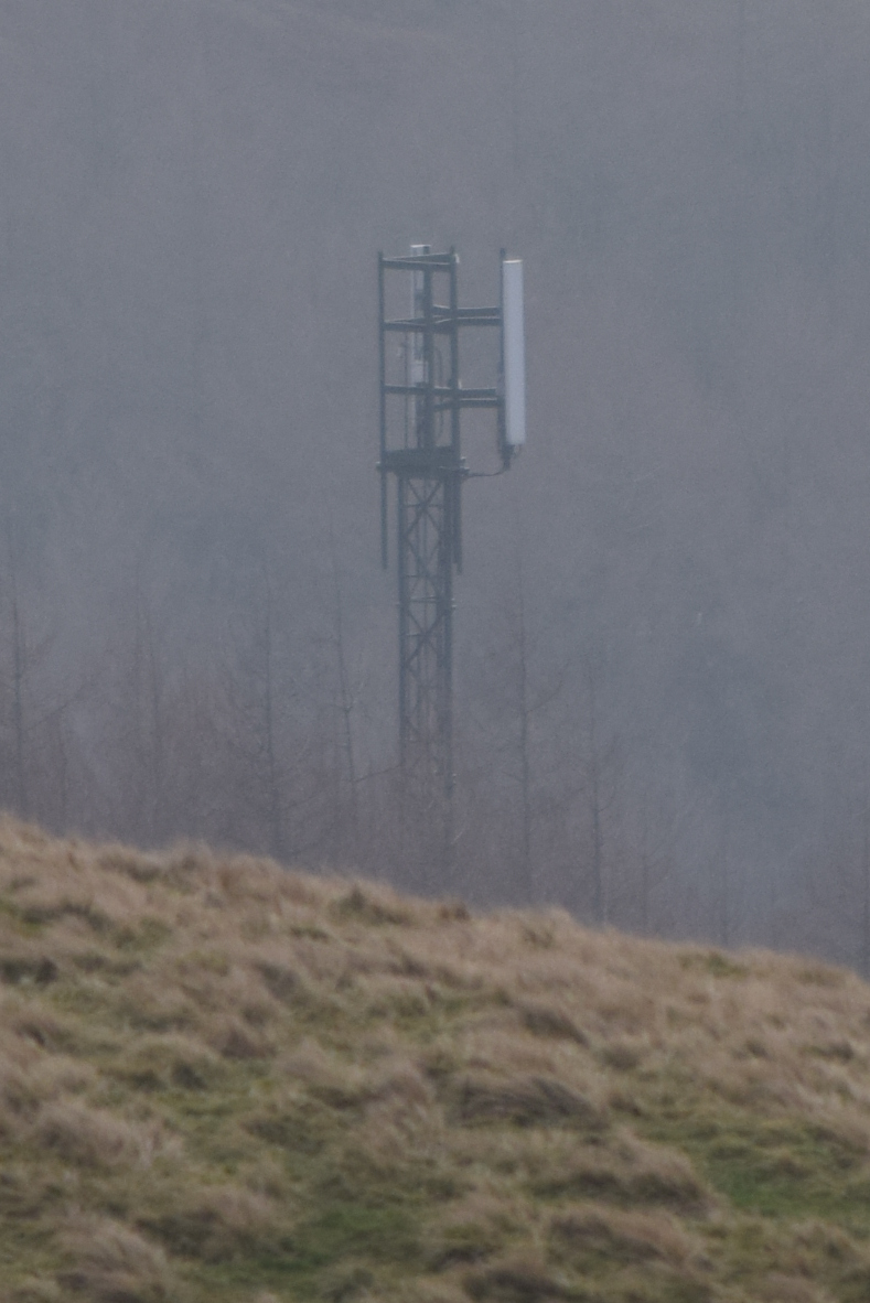
At the top of the hill we could see the target tower’s directional panels which confirmed it was configured to serve the A57 “Snake pass” road below. One panel was oriented north-west towards Manchester (CID 130256660) and the other south-east towards Sheffield (CID 130256650). Based on the dimensions of the panels we estimated their beamwidth as at least 120 degrees and gain of at least 10dBi.
As we passed the eNodeB along the hill top we were conscious of a number of cell neighbours and performed a targeted re-selection where we ended up briefly attached via the antennas back-scatter of *6650, made possible by our proximity. This didn’t last for long before we re-selected to a strong signal (PCI 337) which we were convinced was CID *6660. It wasn’t. Surprise number 2.
We later found out this was also a distant cell with line of sight near Hope, 7km due south of us!
Marching on happily with a great signal, we started a gentle descent until we lost the horizon behind us. At this point the neighbours we observed disappeared and our serving cell (in Hope) became very weak as we entered the signal’s (diffracted) beyond-line-of-sight (BLOS) shadow. As predicted in the video based on the surrounding high plateau we could see, we lost the signal as we continued to head north toward Alport Castles, a local feature. We descended into the valley below without a signal (despite a national map suggesting otherwise) and continued the next 3.5km without any coverage at all 🙁
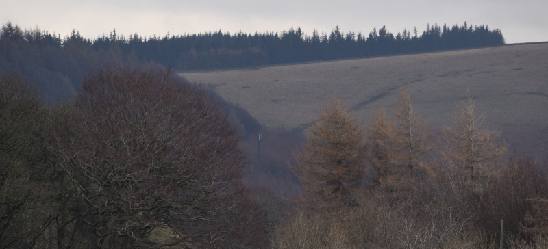
As we exited the remote valley, heading towards the A57 road, we reacquired a signal and finally locked onto our target, *6660, with an excellent signal and line of sight (Credit to Chris for spotting the tower in the trees at 2.7km!). As observed, the directional pattern was focused on the road and we were in the main beam.
A quick map study and we elected to march west until we lost the signal. This event occurred after only 1.5km thankfully as we hand railed the road over undulating terrain. We followed the same route back to the acquisition point which doubled our measurements for this section.
From the A57, in the main lobe, we climbed the hill to the south east and headed back toward the target cell. Knowing it had a directional pattern, we anticipated signal strength decreasing as we exited the main lobe which we confirmed as we drew parallel with the cell, eventually circumnavigating it to the south.
As we exited the beam of *6660 and entered the influence *6650 we re-selected for the final phase of our journey which would take us into a steep ravine and then up the hill, right past the cell.
A sweaty climb up a steep hill behind the cell, saw signal strength and field testing enthusiasm collapse which was fixed with some fizzy snakes. We lost the cell for good only 500m behind it due to the convex hill and directional pattern.
Moral of the story is, in RF, proximity to an access point is no guarantee of service!
Serving cells
| Cell ID | PCI | Location | Technology | Frequency | Comments |
| 130256650 | 272 | Hagg Farm (South East) | LTE Band 20 10MHz | 806MHz DL | ~15m AGL |
| 130256660 | 270 | Hagg Farm (North west) | LTE Band 20 10MHz | 806MHz DL | ~15m AGL |
| 131377930 | 337 | Hope Quarry | LTE Band 20 10MHz | 806MHz DL | ~15m AGL |
| 131413770 | 441 | Little Hucklow | LTE Band 20 10MHz | 806MHz DL | ~20m AGL |
The cells all have a downlink and an uplink frequency. As these four cells share the same downlink they are separated in time using a multiplexing schema and the Physical Cell Identifier (PCI) code. If we only took out a spectrum analyser we’d never know which cell we are looking at otherwise.
Data analysis
We chose to model after field testing. We could have done it before but it would have ruined all the surprises that came up during analysis like the serving cell 13km away!
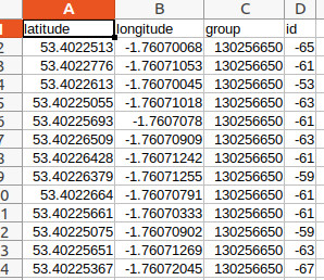
We extracted the CSV data (1034 rows) from the survey tablet which for cell mapper was located at /storage/emulated/0/Android/data/cellmapper.net.cellmapper/files/.
We sorted it by cell and created clean CSV files for each cell with only the location and RSSI.

Gap analysis
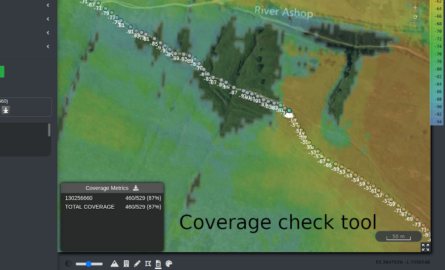
We used our new “coverage check” CSV import tool. This tool allow the import of customer locations which can be tested against visible coverage layers to report a correlation.
This is a binary yes/no comparison with a summary report eg. “87% coverage” which is handy for comparing options.
It cannot automatically calibrate field test measurements but is useful for gap analysis as a “first pass” toward calibration.
This tool is handy for manually aligning the modelling until it matches visually but is too simplistic for calibration.
Fine tuning inputs
Our confidence level for the inputs started around 50%, based on known frequencies, heights and power levels for the UK network. For the first cell, we used a combination of known, observed and assumed values.
You can be forgiven for thinking why not do field testing with known transmission parameters but even then you must calibrate as old batteries, weathered connectors and battered antennas will all impact a transmitters actual effective radiated power (ERP).
As we working LTE800 we used the ITM model, designed for this UHF band when it was conceived for TV broadcasting. This general purpose model has built in diffraction and also has a reliability variable which we can use for fine tuning.
Known values: frequency, location, approximate height, approximate azimuth
Estimated values: Antenna azimuth, beamwidth, gain, RF power, exact height
Once we had a coverage plot using some sensible power values and the coverage-check tool reported a correlation > 90% we rendered it using the Greyscale GIS colour schema and download a GeoTIFF raster. This contains fine grain signal values to 1 dB resolution.
Calibration process
We suggest this workflow for the calibration process.
We also have an API capable of returning data in open vector and raster formats including SHP and GeoTIFF so there are other ways to do this...
- Gap analysis with the coverage check tool in the web interface and approximate/rough inputs
- Power balancing with the path profile tool for selected points only (Recommend a LOS link at long range)
- Gap analysis with the coverage check tool in the web interface and power balanced inputs
- Regenerate the layer with the GIS schema and export for precision offline calibration
- Make minor (1-2dB) adjustments to either the loss or gain values for LOS links, and/or clutter profiles for BLOS until the calibration script reports an RMSE value < 10.
Offline calibration
Using a Python script and the rasterio library we were able to query each row from the CSV data against the GeoTIFF raster instantly, negating the need for many recursive API calls.
The offline method is more efficient when working with large point-to-multipoint layers and spreadsheets than calling the API directly. It computes a mean error which can be positive or negative and a more useful root mean square error (RMSE) which is always positive. A lower figure is better with 0dB being ideal (and also impossible).
The API method is still valid for testing select points or calibrating dynamically.
python3 Offline_Calibration.py 131413770.csv 131413770.tiff
...
Lat: 53.402250 Lon -1.760703 Measured: -65.0dBm Modelled: -68.0dBm Error: 3.0dB Mean error: 0.5dB
Lat: 53.402252 Lon -1.760699 Measured: -59.0dBm Modelled: -68.0dBm Error: 9.0dB Mean error: 0.6dB
Lat: 53.402253 Lon -1.760699 Measured: -61.0dBm Modelled: -68.0dBm Error: 7.0dB Mean error: 0.7dB
Lat: 53.402252 Lon -1.760698 Measured: -63.0dBm Modelled: -68.0dBm Error: 5.0dB Mean error: 0.8dB

Model error is mean 0.8dB, pure RMSE 5.6dB based upon 84 measurements
Receiver measurement error: 3.1dB
RMSE adjusted for receiver error: 2.5dB
The modelling inputs are excellent.| RMSE | Description | Comment |
| 0 to 3 | Excellent | Calibrated! |
| 3 to 6 | Very good | Inputs are very close. Fine tuning needed. |
| 6 to 9 | Good | Inputs are good but more tuning needed |
| 9 to 12 | OK | Inputs are OK but not tuned |
| > 12 | Bad | Inputs are bad. Check basics eg. Height, Frequency, Power |
The results
We achieved results better than expected. We were aiming for under 6dB RMSE and achieved 3dB, at 7km range, which is excellent, and coincidentally as accurate as the measurement accuracy of our survey device.
Manual calibration can be time consuming, and collecting good data definitely is. We felt we could have improved the scores further with more data, like the antenna data sheets for starters, but were happy with our 3dB.
The good
The best results came from the distant cells where LOS was achieved. This makes sense as without obstacles to complicate things the path loss decays at a predictable rate, based on wavelength, which can be plotted as a clean curve. Once we had this power balanced using the path profile tool and manual adjustments, it produced a great match with the data due to the open nature of the high plateau.

The ugly
The other cells, like our target at Hagg Farm (South east), served a more complex piece of ground in the valley which had steep ravines and tall trees. As expected we didn’t fair as well here and achieved 10dB RMSE. Analysis of where we lost accuracy can be summarised as follows:
- Trees. We found 2m LiDAR to be too conservative here as this contains the tree canopy. We tried smoother DSM with clutter profiles which gave a better result but didn’t go as far as adjusting our clutter profile. This is a future trees blog!
- Proximity. Counter-intuitively, being closer to the cell is not better for measurements and calibration than being further away. This is due both to the way path loss decays on a curve and the highly directional panels cells use. Small differences near a cell produce large differences in data, compared with very small differences up on the plateau with the distant LOS cells. We can model directional panels but are guessing what the *actual* beamwidths are.
| Cell | Points | Mean | RMSE | |
| 130256650 | 164 | -0.7 | 9.8 | |
| 130256660 | 460 | 0.9 | 6.9 | |
| 131377930 | 127 | -1.6 | 3.0 | |
| 131413770 | 84 | 0.8 | 2.5 | |
| TOTAL | 835 | -0.15 | 5.5 |
Look forward
The so what of all this is we have proven the software is capable of high accuracy, given the right input, and we have identified areas to improve it further.
- We will be adjusting our LiDAR to soften it in areas where this is available to fully exploit recent developments with our custom clutter profiles.
- We will be integrating recent developments with offline calibration into our user interface to make this manual process smoother, simpler and faster.
- We will work on automating calibration. Some might call this machine learning blah but it’s just software.
Expect another field testing blog all about……trees.

Scripts and data
You can download our field test data and Python scripts here as well as Google Earth KMZs showing the route,cells and measurements.
