In this study we look at modelling long range microwave links and the key parameters which help get the best out of mobile microwave terminals. When sited properly, a low power microwave terminal can communicate over 100km. When sited badly the same terminal can fail to communicate 5km…
A brief history of microwave
Commercial terrestrial microwave links spread in the 1950s during post-war radio innovation and are used today as backhaul in many key public and commercial networks. A microwave station typically consists of a large tower on high ground with round parabolic dishes communicating in UHF (300MHz) bands and above. As Wi-Fi spread after the millennium, outdoor fixed wireless access (FWA) terminals for long-range (>2km) consumer wireless links became increasingly popular, especially around ISM bands, but only recently have portable tracking terminals like the AVwatch MTS become available, intended for mobile ground to air use at distances exceeding 150km.
The theory
A microwave link is designed to be high capacity and focused in order to carry a large amount of information from one point to another. For this reason they need a short wavelength so are found in UHF and SHF bands above 300MHz.
The signal has a fresnel zone around it which is sensitive to obstructions. Achieving a line-of-sight link is not a guarantee of a good connection if the fresnel zone is obstructed by trees or buildings. The size of this zone is inverse to the frequency so a higher frequency has a smaller zone, akin to a laser beam, compared with a lower frequency which has a larger zone and so requires to be higher above the earth to clear it.
Radio horizon
The maximum distance a microwave link can go over the earth has little to do with RF power and much more to do with the dish heights and the horizon which limits how far a (short wavelength) signal can go. Whilst refraction can extend a link beyond the horizon, it is variable like the weather so impractical to model accurately and in a timely fashion. A simple formula to calculate the radio horizon is 4.12 x sq(height) where height is the combined transmitter and receiver altitudes. This formula produces a table of horizons which show that an improvement in height of several meters translates to a range improvement of several kilometers due to the earth’s curvature.
| Transmitter height m | Receiver height m | Radio horizon km |
|---|---|---|
| 1 | 1 | 6 |
| 1 | 10 | 14 |
| 1 | 50 | 29 |
| 1 | 100 | 41 |
| 1 | 200 | 58 |
| 1 | 400 | 82 |
| 1 | 800 | 116 |
| 1 | 1600 | 164 |
Parabolic antennas
As signal attenuation is substantial at these frequencies they require a highly directional antenna to improve forward gain and cancel noise from other angles. The larger the dish size the greater the gain and the smaller the beam.
A microwave dish antenna is easily recognised as a polar plot by it’s prominent main lobe, symmetrical side lobes and minimal back scatter. It has a very high front-to-back ratio which describes the ratio of forward power to rear in the order of +50dB. Due to it’s high directional gain it only needs to be driven with a modest amount of RF power to generate an effective radiated power of several hundred watts.
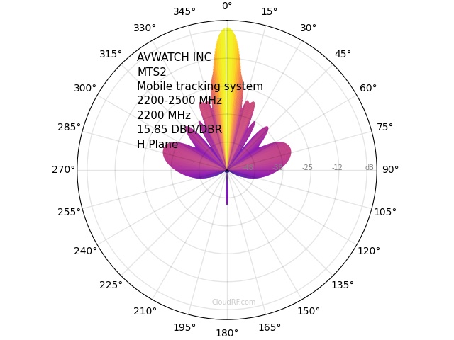
Parabolic polar plot (Azimuth) 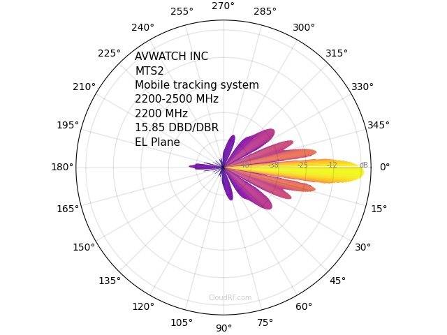
Parabolic polar plot (Elevation)
Using and creating a directional pattern
In CloudRF you can choose from thousands of crowd sourced patterns, upload your own in TIA/EIA-804-B / NSMA standards or create your own using a few parameters.
To select a template, open the Antennas menu in the web interface and click the database icon. This will open a search form. Search by manufacturer, eg. Cambium, or model. When you find a pattern you want click the green plus symbol to add it to your favourites list. You can now proceed to set the azimuth and tilt as if you were affixing it to a pole.
If the pattern does not exist, you can choose to use a “custom pattern” and define the horizontal and vertical beamwidths in degrees as well as the gain and front-to-back ratios in decibels to generate polar plots. These can be downloaded as a legacy .ant text file which you can upload in the service as a private pattern. A custom pattern is quick to self-generate but lacks side lobes and the full accuracy of a detailed pattern from a manufacturer.
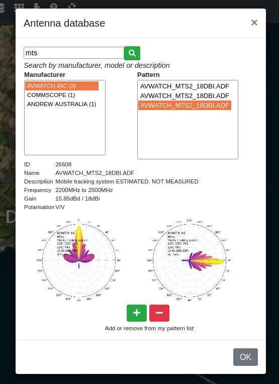
Antenna database 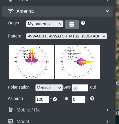
Selected antenna 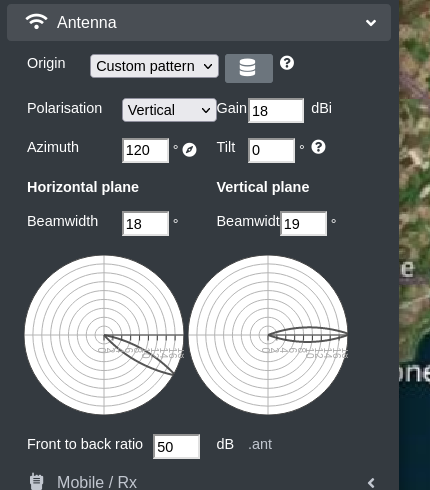
An over the horizon link
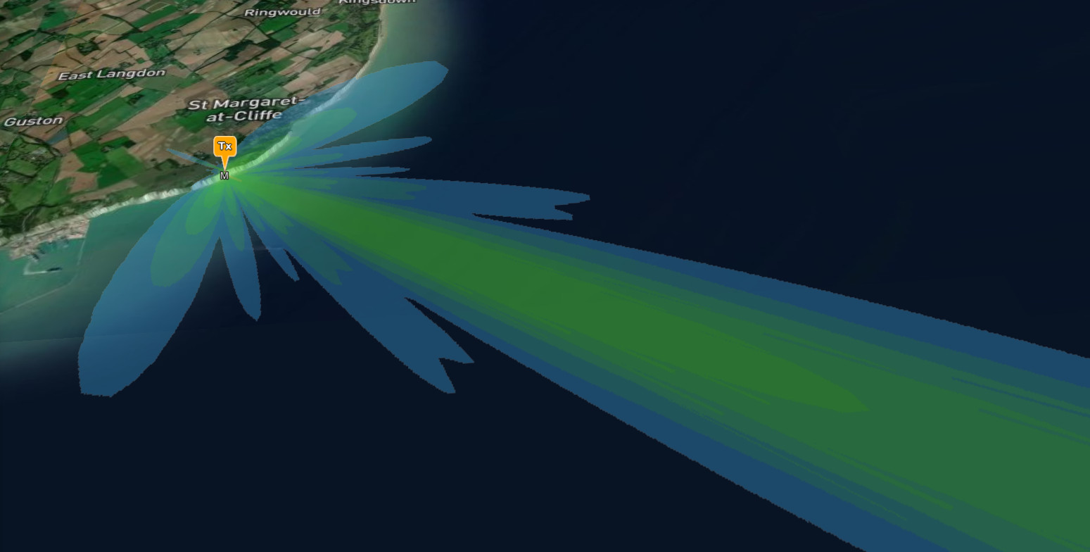
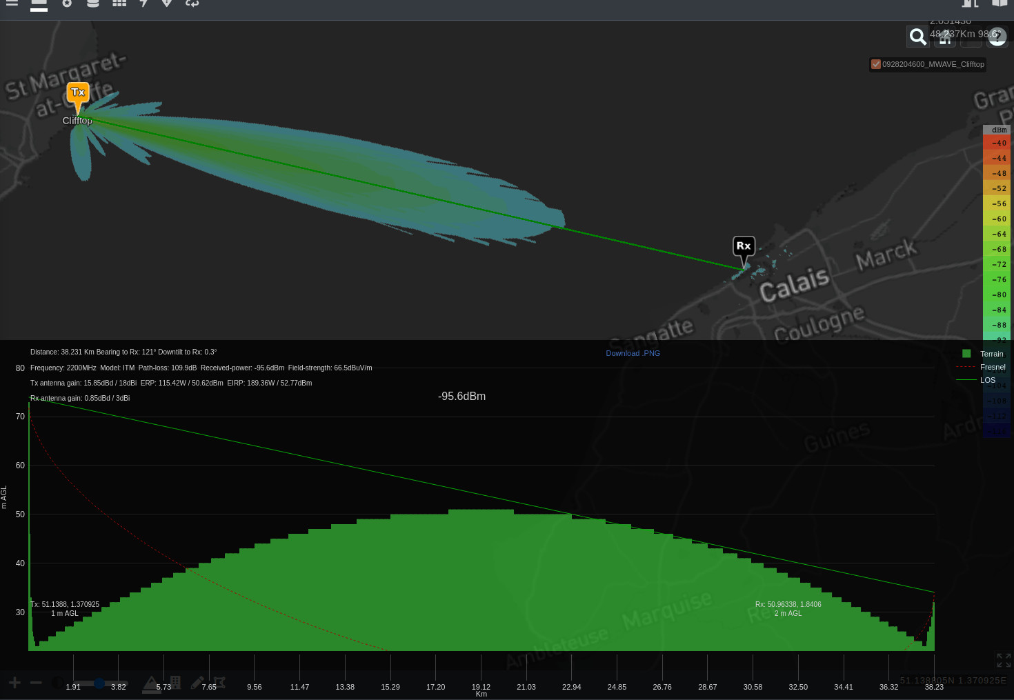
For this demo, we’re simulating a link from the cliffs of Dover in England across the English Channel to Calais, France, a distance of 40km across the sea with no obstructions. The 18dBi terminal is 1m off the ground and is using only 3 Watts / 34.7dBm power for a total effective radiated power of 189W / 52.8dBm. A receiver threshold of -100dBm was used. This is too low for high speed waveforms but would be ok for a telemetry fallback waveform like QPSK.
A bad link
With a ground receiver on top of the cliff, the link just reaches Calais. It is obstructed on the radio horizon at ~25km, a full 10km before the coastline but the height advantage of the cliff makes line of sight just possible to some parts of the town. Despite just achieving line of sight, this link would still be unsuitable due to the majority of the fresnel zone being obstructed.
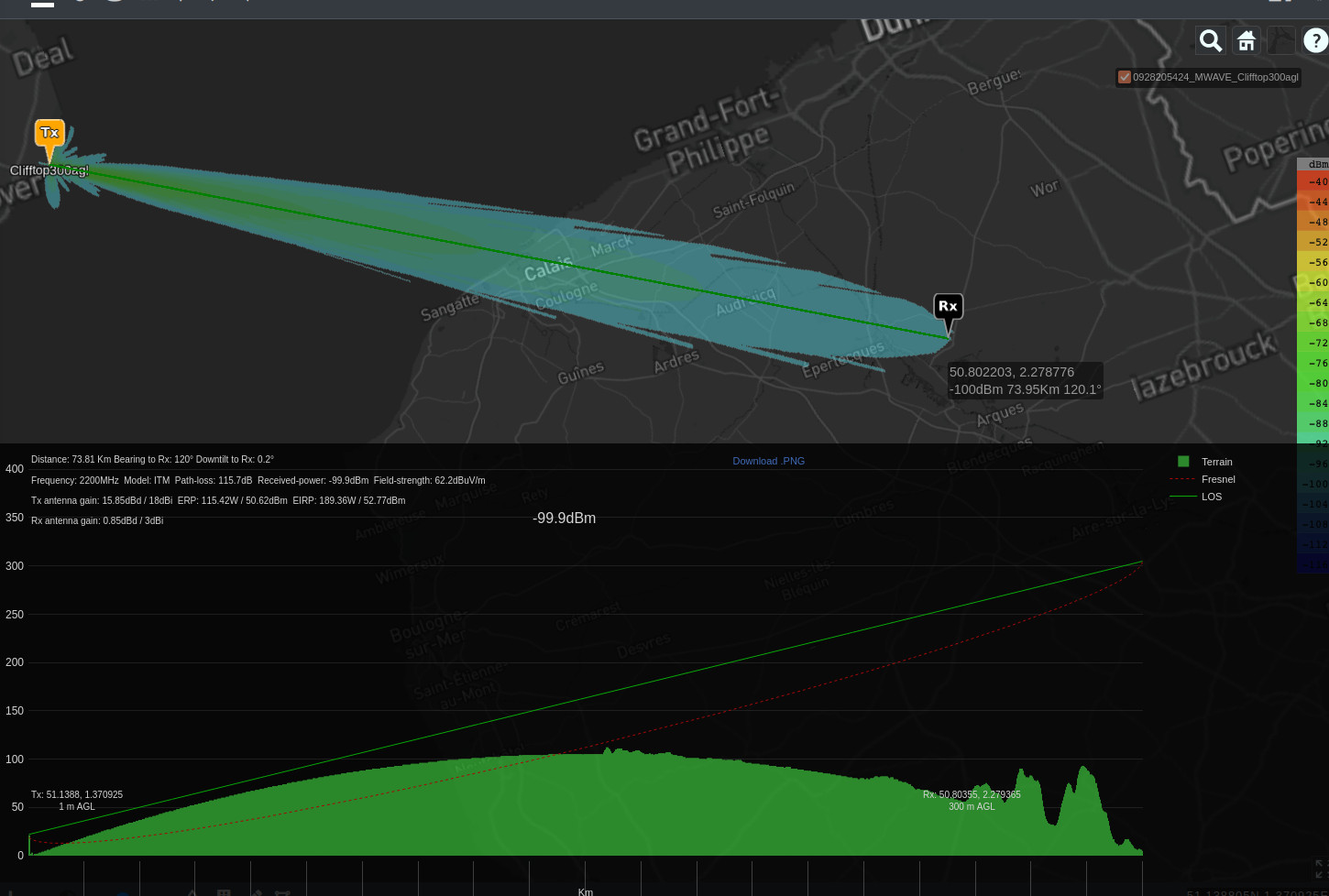
A good link
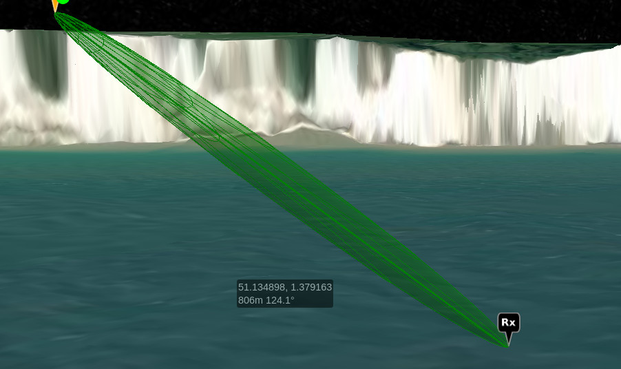
With the same cliff top terminal and RF parameters, the distant receiver is swapped for a drone 300m above the ground. The increase in height extends the link from ~25km to 75km, deep into France with good LOS.
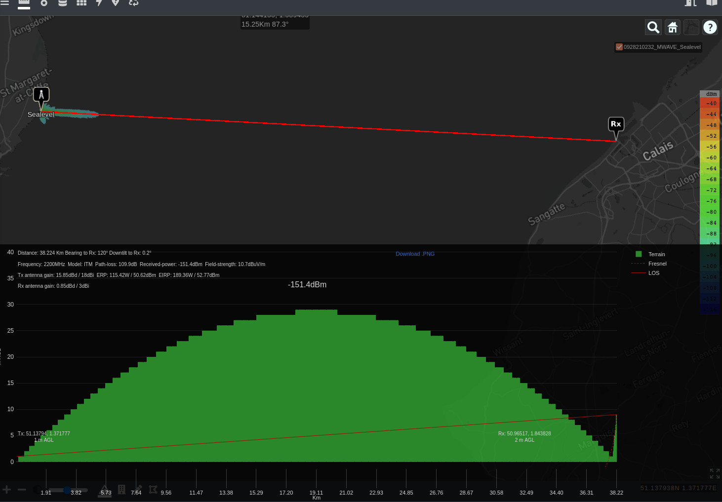
An ugly link
This time the same terminal which just achieved 75km was misused down on the beach to communicate with a small boat in the channel. It’s effective range was less than 6km due to the radio horizon. As you can see from the normalised path profile chart below, the curvature impact is substantial when the stations are on the earth!
Thresholds and modulation
The simplest way to limit the modelling is with received power measured in decibel milliwatts. In this common scale, -100dBm is a sensible threshold for most digital systems. For planning purposes, a 10dB fade margin should be added for a -90dBm threshold. The actual thresholds needed will vary by systems and waveforms. Many commercial microwave links operate very high symbol rate modulation schemas which need received power above -70dBm to function.
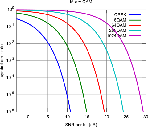
You can also use Bit-Error-Rate (BER) as a threshold. This unit is used in conjunction with the noise floor and the desired signal-to-noise ratio (SNR) to derive a threshold. A modulation schema like QAM64 requires a relatively high 15dB SNR compared with 5dB for QPSK which can function on weak links. These thresholds are not absolute which is why we set the desired error rate. Errors are inevitable and the relationship between the BER and SNR is best visualised as curves. If you know you want QPSK for example but are not sure what error rate to use, use a mid level error rate such as 10-3 (One bad bit for every 1000 bits) which will give you a 7dB SNR. If the local noise floor is -120dBm your equivalent receiver threshold is a pretty low -113dBm.
Conclusion
Forget RF power, height is everything in creating a successful microwave link. This might mean moving a terminal several kilometers away from the distant station in order to gain a few meters in height but the benefit will be many more kilometers in range.
