Cognitive radio, in it’s present form, describes a spectrum sensing radio which can change channel to avoid noise. This capability is standard now on domestic Wi-Fi routers.
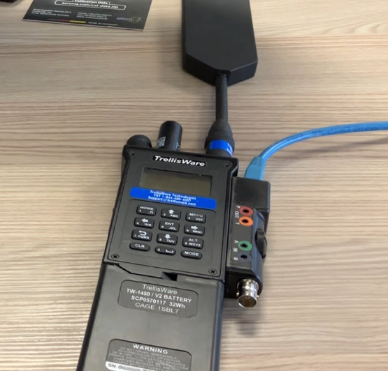
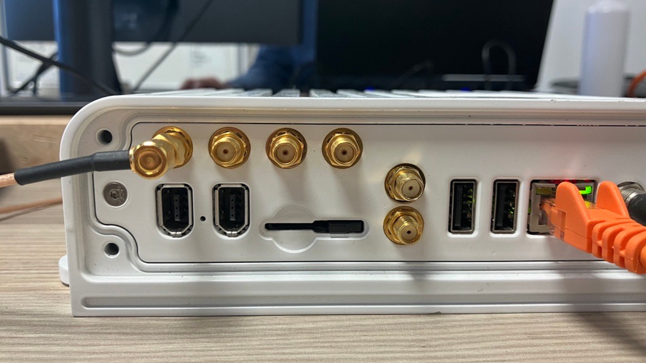
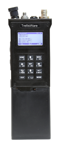
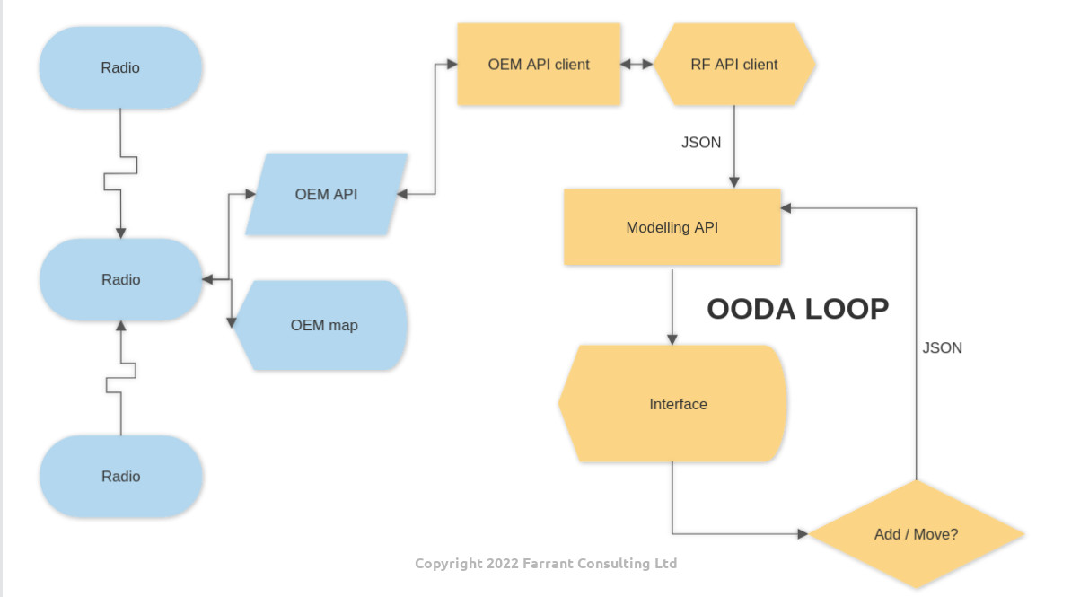
With our modelling API and modern radios with APIs we can do much more. Here we present two demos using a raspberry Pi as the server. By compiling our API for ARM and hosting it on a small computer we negate the need for a network to use the API which means we can develop functions to assist radios which may have fallen off the network.
Dynamic transmit power
Problem
Automatic Gain Control (AGC) is an established concept which uses a feedback loop to adjust power to maintain a desired level. This technology is what makes a mobile phone battery last so long. When the phone is near a tower it radiates a fraction of the power it would if it were far away in the countryside. It’s able to do this as the network infrastructure is fixed and there is a signalling channel to make these adjustments eg. “reduce power 10dB”.
A terrestrial broadcast radio network is a much more dynamic environment and as a result it’s common for radios to transmit more power than they need to as power control is simple (low, medium or high on a dial) and once a radio is set to high, the operator is not incentivised to change it as “it works”. This inefficiency reduces battery life and creates excess spectrum noise.
Solution
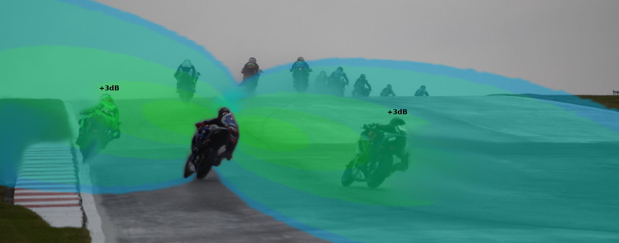
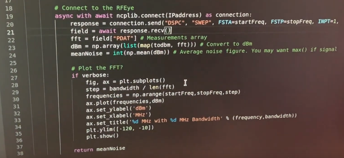
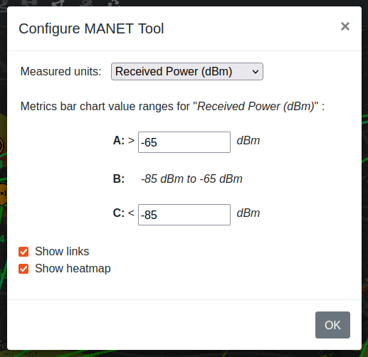
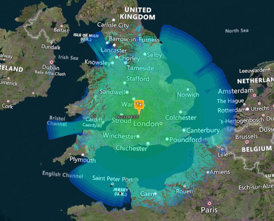
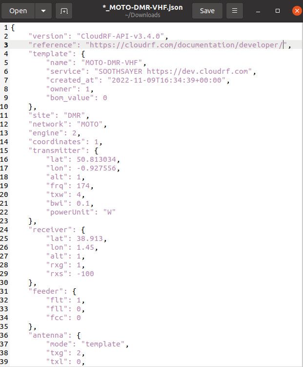
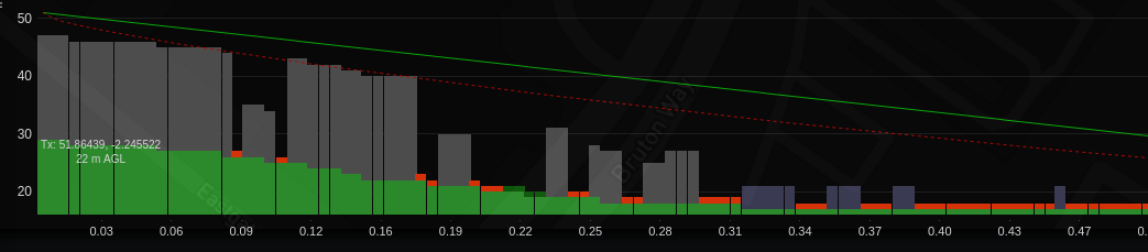
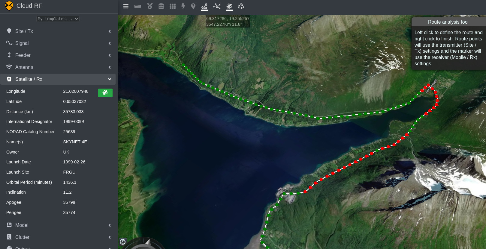
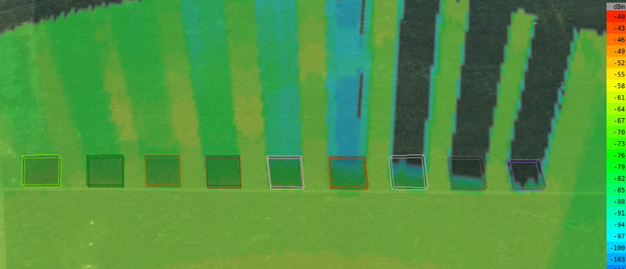
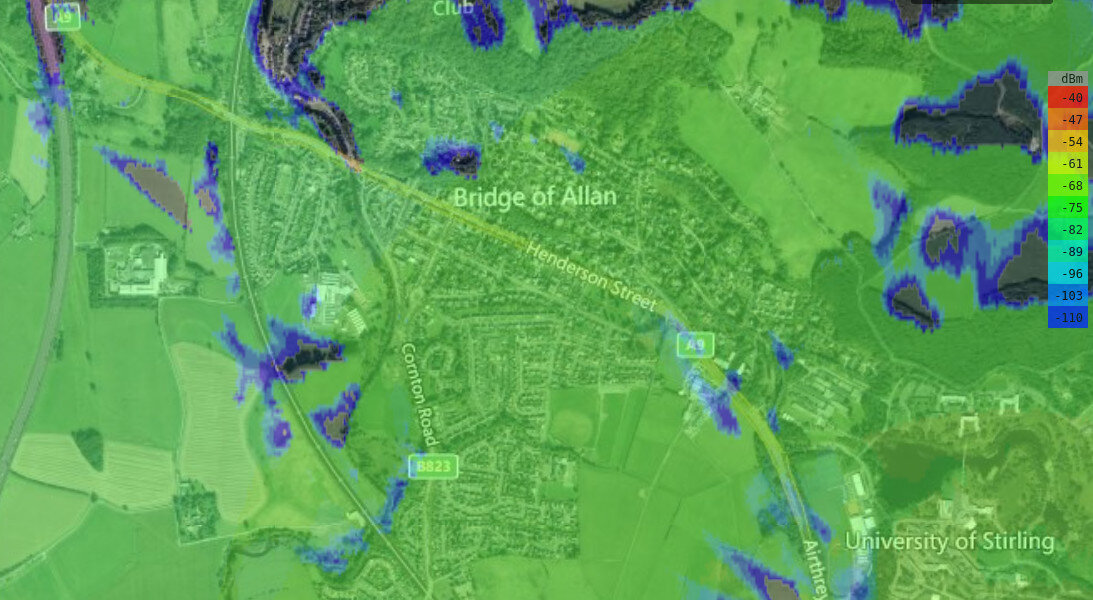
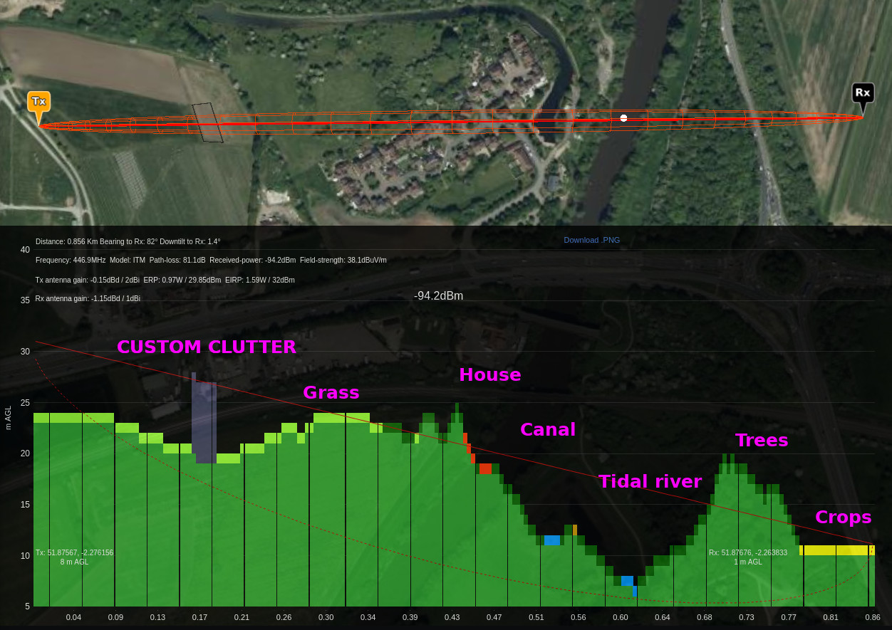
Using our “Path” API, we perform tests to a distant station to establish the modelled signal to noise (SNR) ratio. This distant station could be the nearest node or a repeater. With the SNR result, we are able to compute an adjustment to the local radio to meet a desired signal level. This could be -90dBm for example.
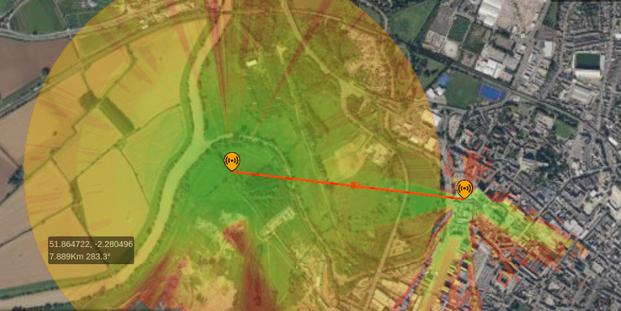
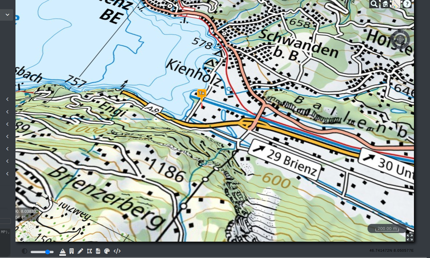
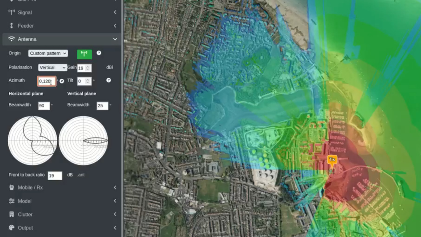
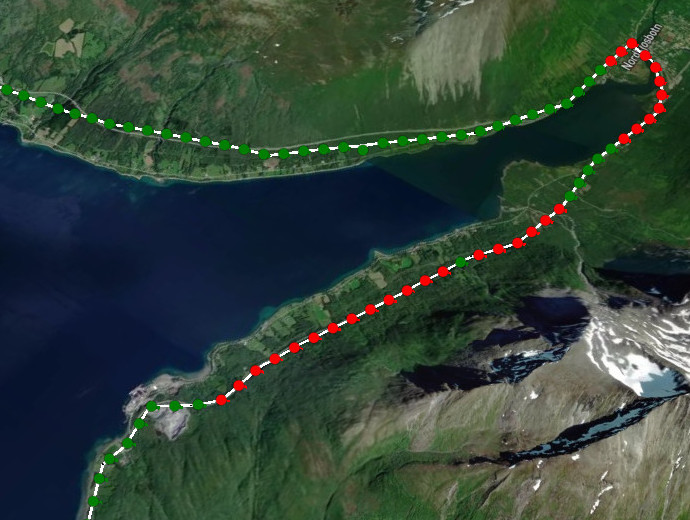
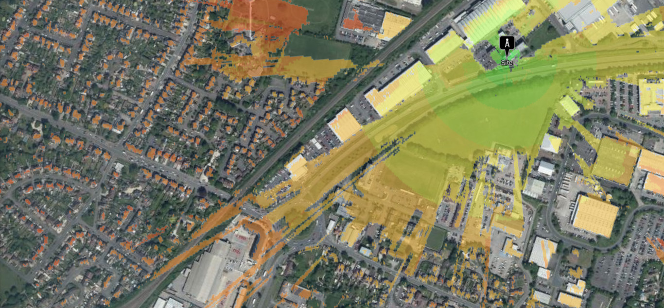
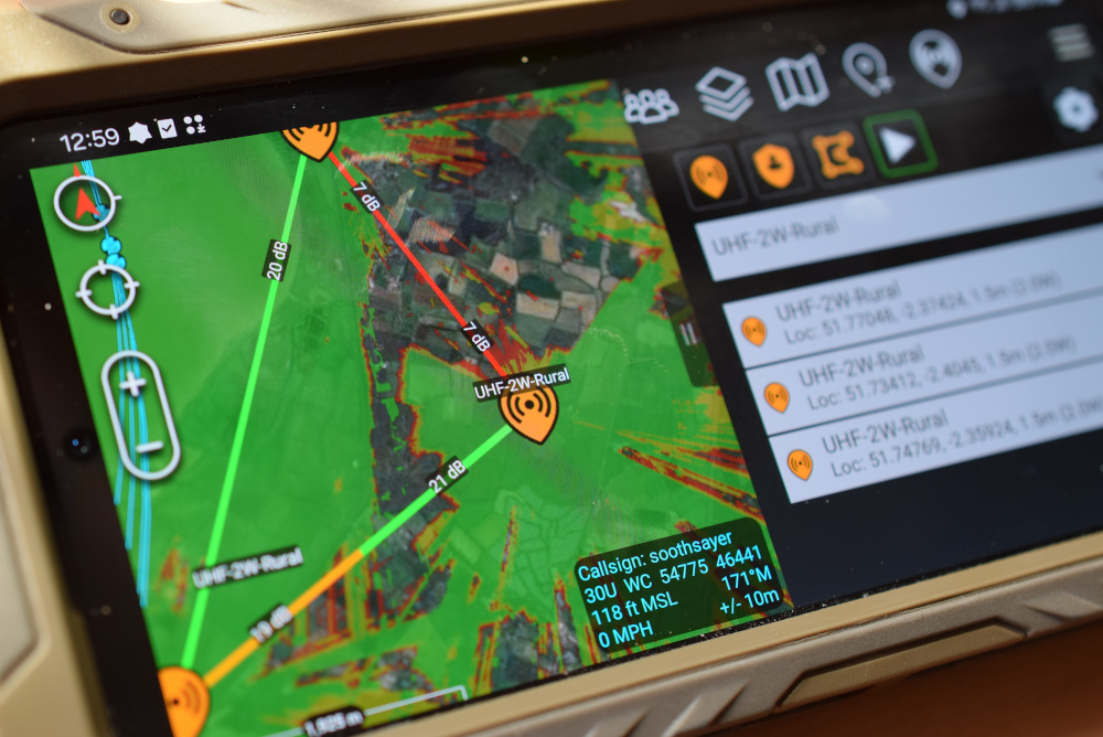
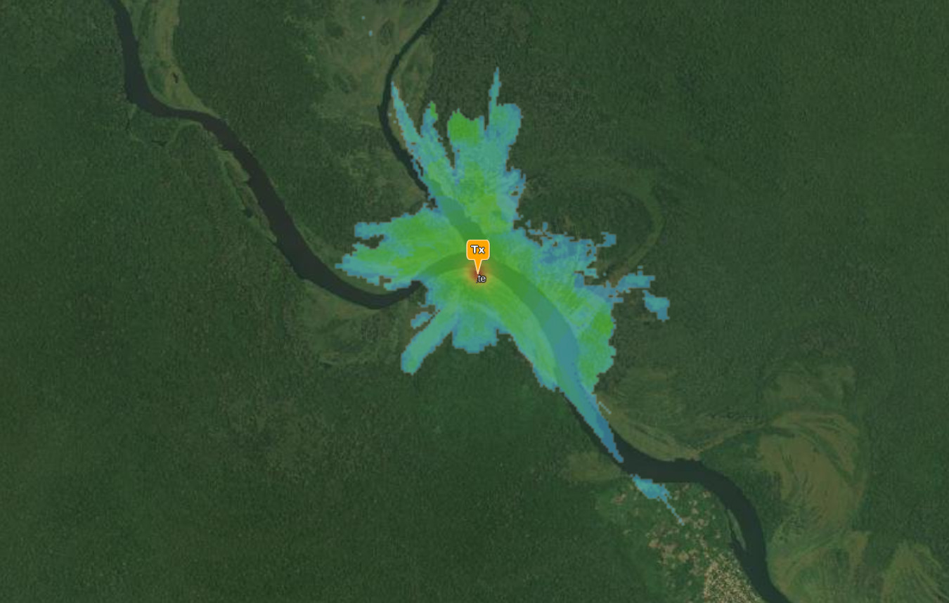
In our demo, we fixed a receiver location 5km west and moved our transmitter on a north to south path through mixed clutter. The variance exercised the dynamic power management up until the transmitter was behind a deep forest and could no longer communicate after which the LCD reported a failure.
Demo source on Github: https://github.com/Cloud-RF/CloudRF-API-clients/tree/master/integrations/AGC%20demo
Best site analysis
Problem
Radio networks have signal dead spots caused by topography like a valley or clutter like buildings and trees. When a VHF/UHF radio operator finds themselves without communication (if they’re aware) they will resort to their training and experience to remedy the issue. These remedies can be technical such as adjusting transmit power, antenna configuration or elevation, all of which will improve a signal, or physical such as moving.
Operators are taught to attempt an initial movement of at least a wavelength (10m at 30MHz) to overcome multi-path effects where out-of-phase reflected signals cause nulls followed by bigger movements. Depending on the scenario, this could easily result in an operator making unnecessary, and potentially risky, movements to acquire a signal. Each movement would be a guess based on local observations of terrain…
Solution
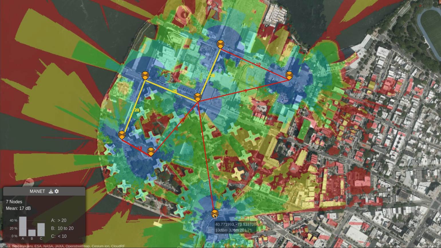
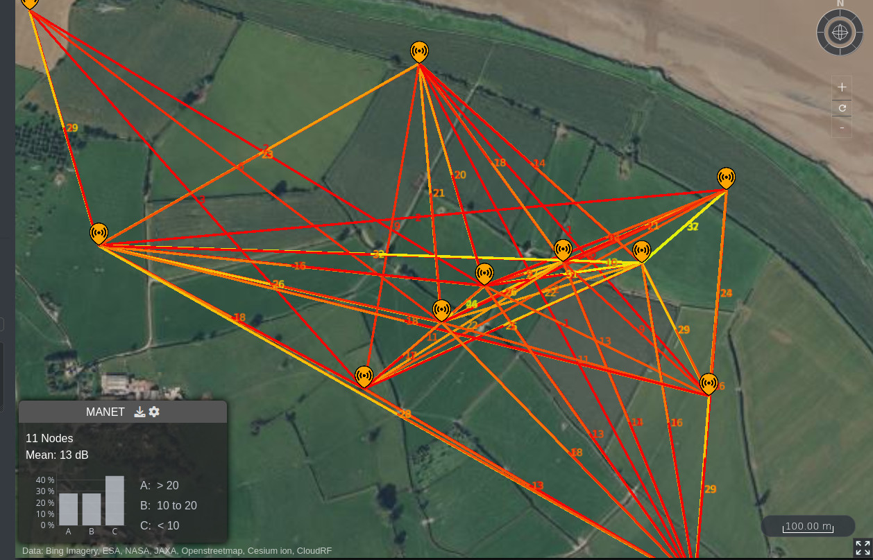
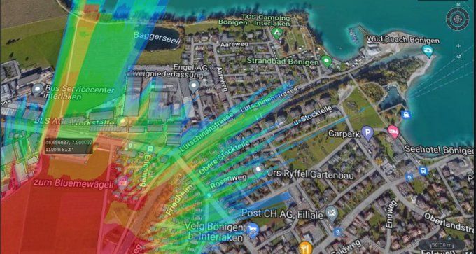
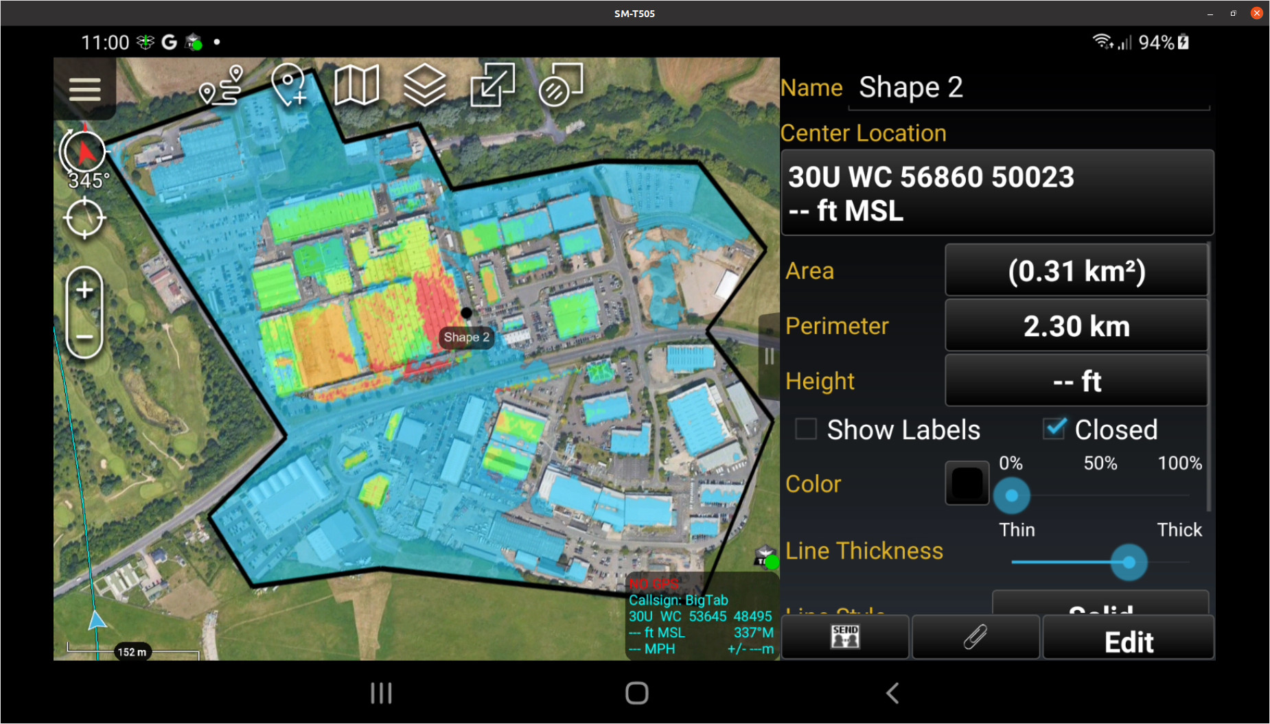
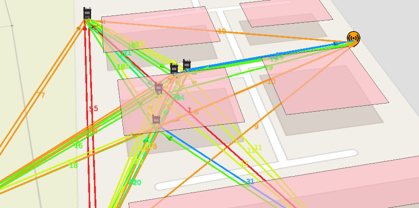
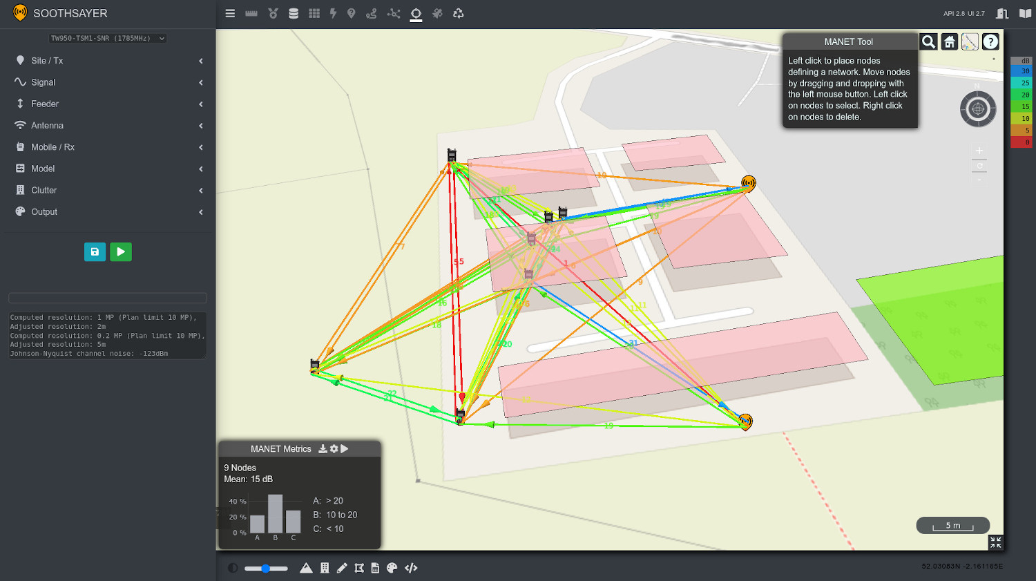
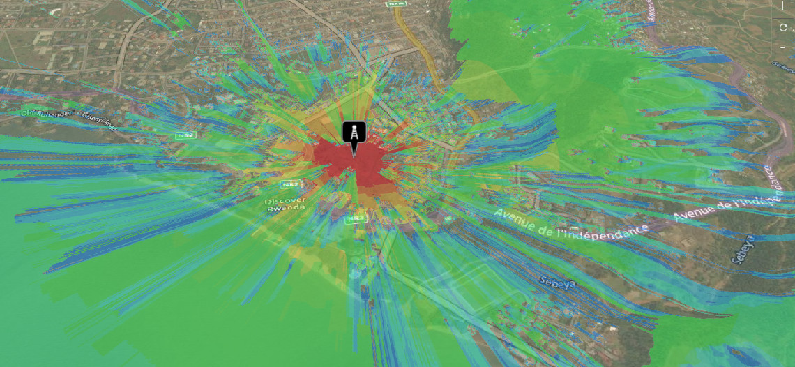
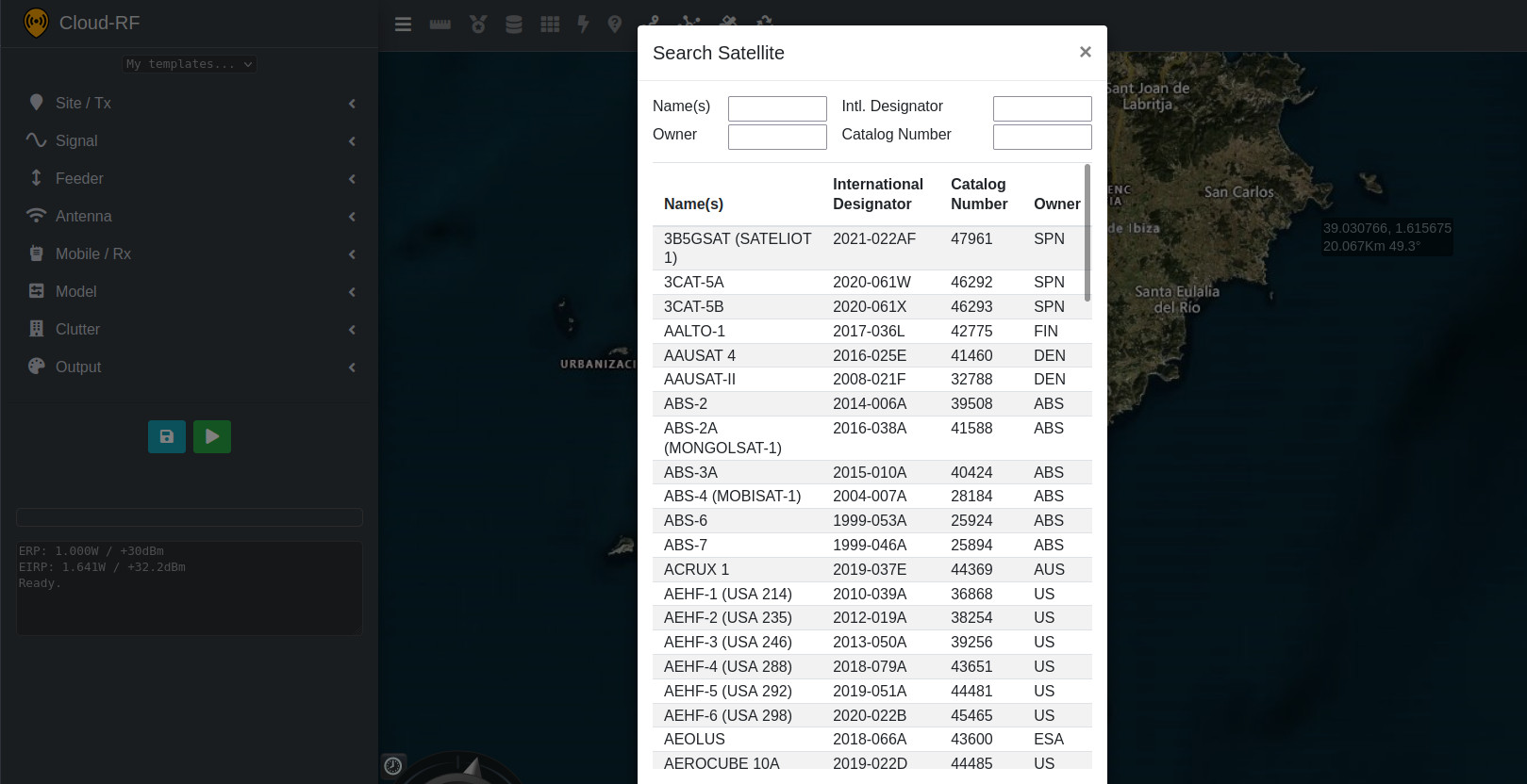
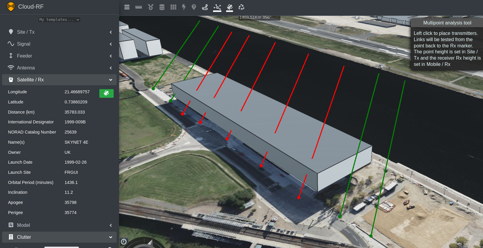
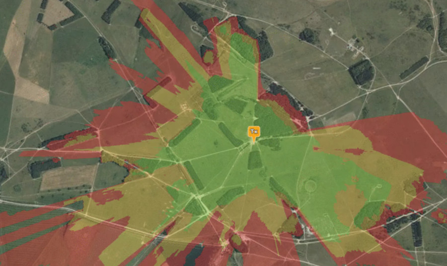
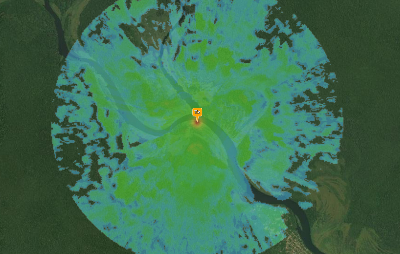
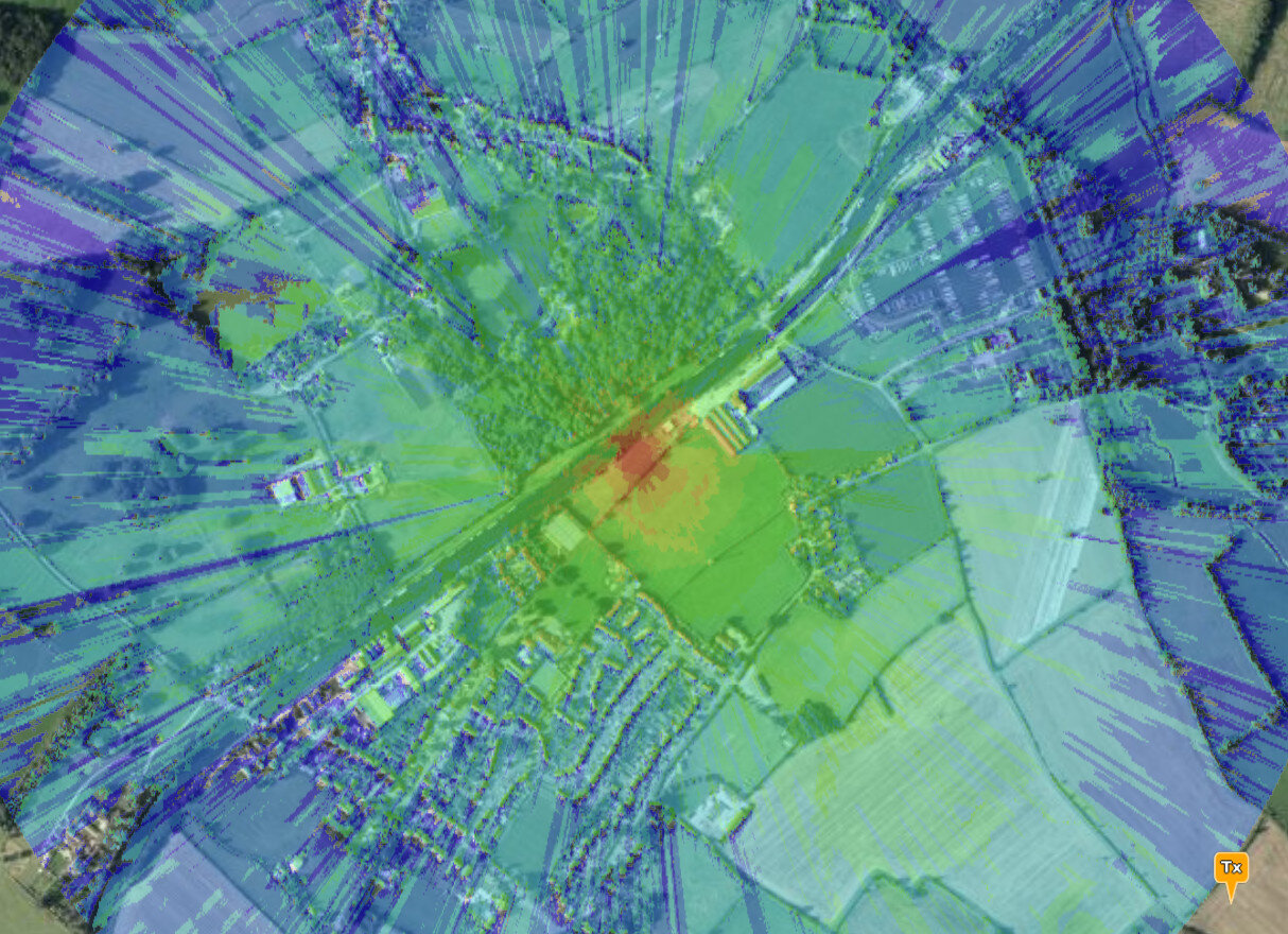
Using our “Points” API, we perform multiple tests in all directions around the radio’s position to a distant station. As before this could be a repeater or a recent neighbour node. The points API is very efficient and takes an array of positions for which it returns an array of simulated values. With this response we can determine the best location to move to.
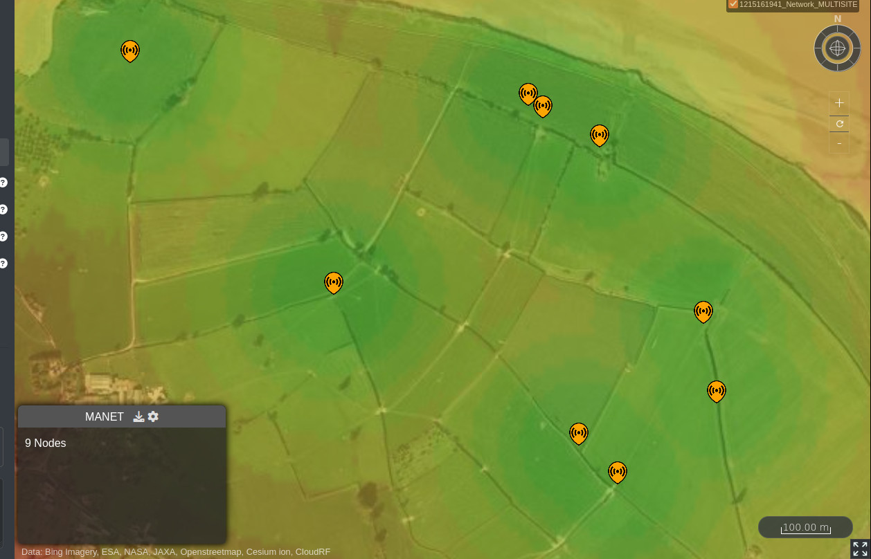
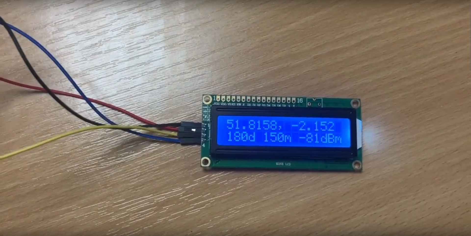
This search is conducted at an expanding search radius until a signal is found. A signal is defined as being above our desired threshold for the system, in this case -90dBm. This result is presented to the operator as a short message composed of a bearing, distance and expected signal strength.
If the operator wants to take control of the search, they can do this using the keypad and virtually walk around the area as a grid. Results for each grid are presented to the operator via the LCD so they can find out if a hill is worth climbing without climbing it.
A look forward
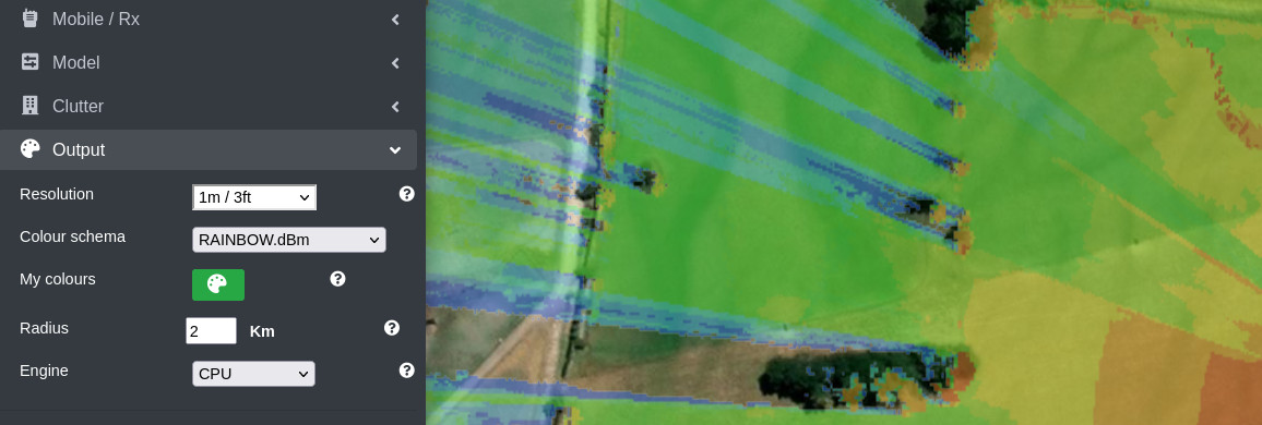
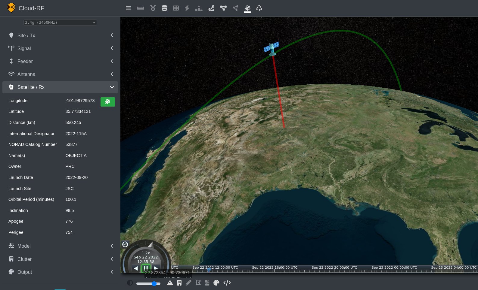
More radios are featuring APIs which allow for dynamic control of the radio, and eventually the network. APIs are the key to enabling a truly cognitive network and we have the modelling API, 11 years in the making, capable of supporting the scale, speed and accuracy needed which can be installed on ARM via a container. As a look forward, we will be installing this on a Samsung S21 where aside from powering our ATAK plugin, we will be able to do powerful modelling capabilities at the edge without a network – or a heatmap.
If you are a hardware OEM interested in enhancing your product please get in touch.