Web Interface Import Data
You can import structured data in different open formats by clicking on the  which is located at the bottom of the web interface. This will open a dialog modal window from where you can select a function to work with.
This modal window is separated into the following sections:
Reference display
Add markers / boundary lines to the map from a KML
Coverage analysis
Import zip codes / locations to study coverage statistics
Route analysis
Import a route or flight path to analyse coverage
MANET network
Import locations from a file to model a network
Survey data
Import field measurements (Lat, Lon, RSSI)
Calibration
Import field measurements (Lat, Lon, RSSI)
Best Site Analysis
Import an area to study it using a Monte Carlo simulation
Automatic processing
Import a spreadsheet of data for processing via the API
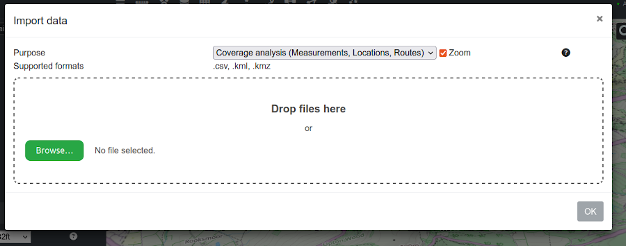
To make use of this tool simply select your chosen “Purpose” and upload your data in one of the specified formats.
At any point if you wish to remove your reference data from the map then you can simply click on the “Clear Layers”  button along the top of the interface.
For more guidance on automatic processing, please consult the dedicated section.
File Validation
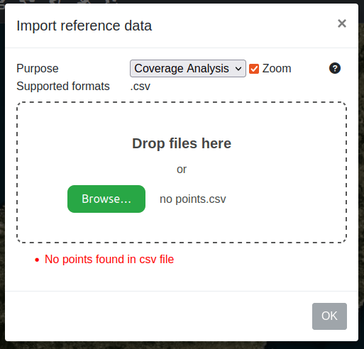
Regardless of the “Purpose” selected, your files will be validated when you upload them. This ensures that your files will work with the interface and be interpreted correctly.
If you have an error in your reference data then this will be displayed in the modal window.
Reference Display (Shapes on the map)
If you select “Reference Display” from the “Purpose” dropdown then this can be used to display imported data on the map such as polygons or pins.
When you select this option from the “Purpose” dropdown this will also show a new colour picker input which can be used to set the colour of your import data when it is drawn on the map.
This functionality can be used to create guides on the map where you can visualise where certain points or boundaries may be. For example, you may upload a CSV of points to indicate important landmarks, or you may upload a GeoJSON file which includes a boundary.
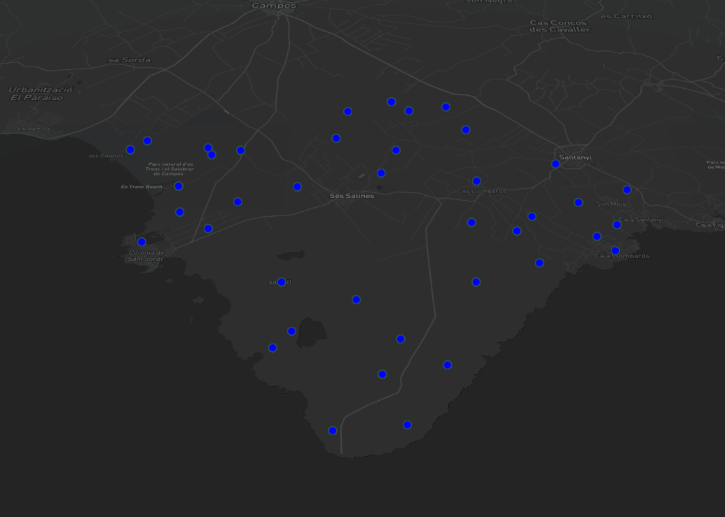
Below shows uploaded points using the “Reference Display” from a CSV:
Below shows a sample CSV which was partially used to produce the above screenshot:
longitude,latitude,rssi
3.0505242,39.2707224,-70
3.0807366,39.2866678,-50
3.0560174,39.304735,-92
3.068377,39.2935764,-90
3.0340447,39.3100479,-67
3.0910363,39.3100479,-75
3.0381646,39.295702,-81
3.0632271,39.2842762,-91
Below shows a boundary uploaded using the “Reference Display” from a GeoJSON file:
Below shows the GeoJSON which was used to produce the above screenshot:
{
  "type": "FeatureCollection",
  "features": [
    {
      "type": "Feature",
      "properties": {},
      "geometry": {
        "coordinates": [
          [
            [
              1.4256018139448656,
              38.92015233473046
            ],
            [
              1.4280509904125438,
              38.91581165124461
            ],
            [
              1.4449950785628118,
              38.91780215762395
            ],
            [
              1.441954782658172,
              38.92844609186906
            ],
            [
              1.4256018139448656,
              38.92015233473046
            ]
          ]
        ],
        "type": "Polygon"
      }
    }
  ]
}
Coverage Analysis (Measurements, Locations, Routes)
If you select “Coverage Analysis” from the “Purpose” dropdown then this powerful utility can be used for several purposes:
Upload field measurements / RF survey data which can be used to calibrate and optimise simulation settings by reporting the error
Upload location data eg. zip / postal codes which can be used to gather metrics about coverage for areas and points.
Upload a KML route for coverage analysis. This will report the percentage (%) of the route covered
Coverage analysis of locations
You can upload a CSV with data about multiple points, for example customer properties by ZIP or UPRN.
For basic ‘points’ your CSV should follow the following rules:
The following fields are accepted:
idis a unique identifier of the point.latitudeis the latitude coordinate of the point. Should be a decimal value between -180 and 180.longitudeis the longitude coordinate of the point. Should be a decimal value between -90 and 90.groupis an optional field which allows you to group certain points together.
Your CSV must contain a header indicating the ordering of your fields.
An example CSV might look something like the below:
id,longitude,latitude,group
Point 1,3.0505242,39.2707224,SOUTH DISTRICT
Point 2,3.0807366,39.2866678,SOUTH DISTRICT
Point 3,3.0520286,39.3742523,NORTH DISTRICT
Point 4,3.0678215,39.3787639,NORTH DISTRICT
After successfully uploading your CSV it will be parsed and the interface will automatically draw your points onto the map.
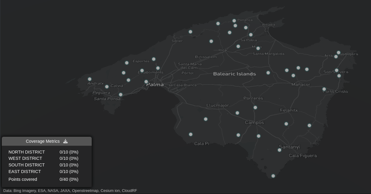
You may notice that a new window will be added to the bottom left of the screen. This is a live-updating metrics report which gives you details about your calculations, giving indications as to whether your points are covered or not.
If you next click on the map and run through a calculation you should see the points being coloured based on the signal strength but also the metrics report should update automatically when new calculations cover points.
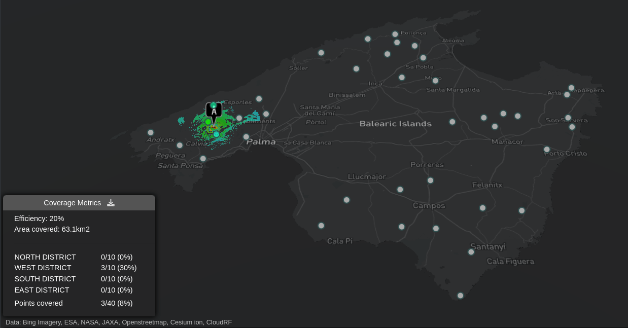
As you add new calculations this will update the metrics report showing you how much coverage you have in total. Each group as defined in your CSV will also be calculated based on its coverage.
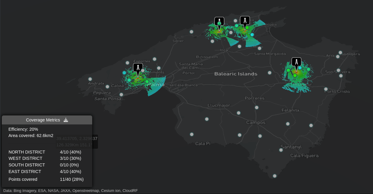
As you do multiple calculations this will build up your available layers on the map. As you check/uncheck them it will automatically update your metrics report in the bottom left of the interface. This is useful for seeing the effect removing a single layer has on an overall network.
In the “Coverage Metrics” window you can click on the “Download Coverage Metrics Report” icon  to obtain a report from your calculations. This is a
 txt file with information:
Location Coverage Metrics Report
Thu Apr 06 2023 12:56:54 GMT+0100 (British Summer Time)
Cloud-RF

NORTH DISTRICT: 4/10 (40%)
WEST DISTRICT: 3/10 (30%)
SOUTH DISTRICT: 2/10 (20%)
EAST DISTRICT: 4/10 (40%)

TOTAL COVERAGE: 13/40 (33%)

Layers:
0406125414_My_Site
0406125639_My_Site
0406125642_My_Site
0406125645_My_Site
0406125651_My_Site
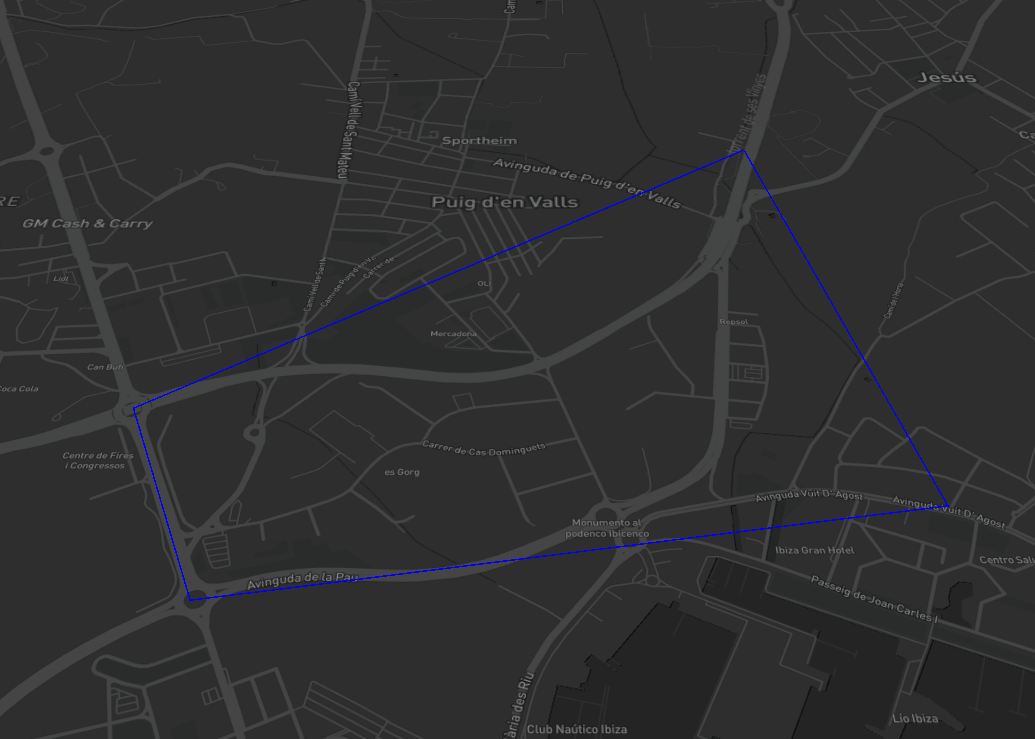
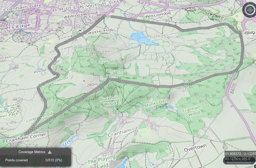
Route analysis
The route import feature lets you load a CSV, KML or KMZ polyline describing a route for analysis. This is a more advanced and powerful alternative to the “route analysis” tool which is only a freehand “quick look” against the start position.
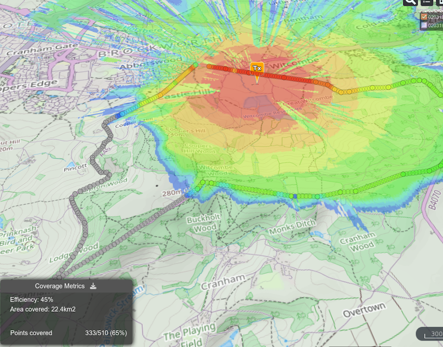
Load in the KML to render it on the map and then create or reload a heatmap layer. This layer can be either an “area” calculation or a multisite heatmap using the MANET tool.
Multiple layers can be added to the map for analysis. When a layer is removed, it is updated.
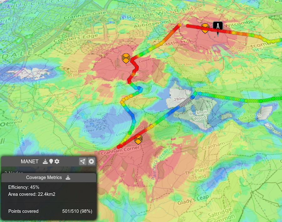
Note that clearing the map at this point will also clear the route so use the layer manager instead to hide layers.
The MANET tool, when used in conjunction with route analysis will update the coverage statistics after every change.
Import a flightpath
The data only needs points for each vertex as it uses interpolation to complete the route. Route coverage is presented in the corner as a percentage against use defined radio parameters eg. 75%.
The route import feature supports flightpaths above the ground as CSV or KML. Both OGC line strings and gx extensions are supported. You can fetch a flightpath from ADSB exchange and load it in directly.
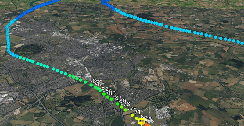
Only one flightpath is supported within a KML file and sometimes ADSB files contain several; for example one for taxiing and another post take off.
Altitudes will be placed using the selected altitude units. If you need height AMSL then ensure you select this.
To test coverage to a ground site, click on the map to site the receiver and click the play button to test the path using the points API.
MANET network
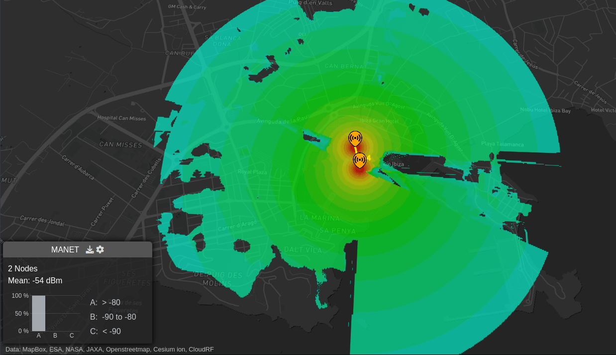
If you select “MANET Tool” from the “Purpose” dropdown then this can be used to import points for use with the MANET tool (GPU required). This is useful when you wish to use the MANET tool but don’t want to have to keep redrawing markers at the same locations if you want to test different profiles for example.
Please note that when you upload your file using “MANET Tool”, each point in your uploaded file will be applied with the same values that you currently have set for your settings.
After you submit your uploaded file a MANET calculation will be fired off immediately using your settings and preferences.
Below shows the result of a MANET calculation after being uploaded from a KML file:
The above screenshot is taken from the following KML:
<?xml version="1.0" encoding="UTF-8"?>
<kml xmlns="http://www.opengis.net/kml/2.2">
  <Document>
    <Placemark>
      <name>Point 1</name>
      <Point>
        <coordinates>
          1.4397022,38.9146682,0
        </coordinates>
      </Point>
    </Placemark>
    <Placemark>
      <name>Point 2</name>
      <Point>
        <coordinates>
          1.440185,38.9130821,0
        </coordinates>
      </Point>
    </Placemark>
  </Document>
</kml>
For more information please consult the section relating to the MANET planning tool.
Survey data and Calibration
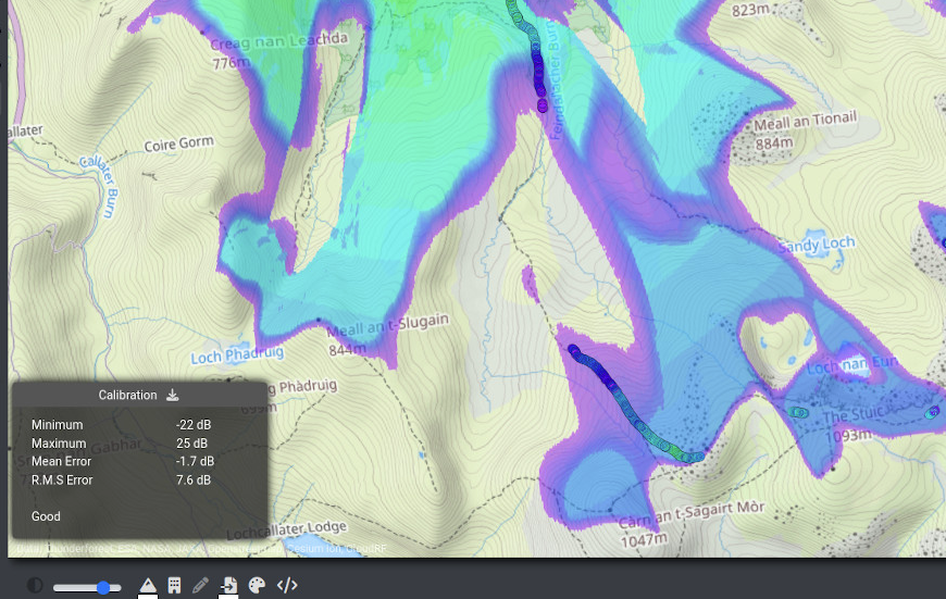
You can upload a CSV with field measurements for easy modelling calibration. This was developed with CSV output from Cellmapper which is recommended for cellular surveys like the LTE800 survey in the image above.
Survey hardware like Nemo Handy and SDRs are also supported providing power measurements can be represented as dB or dBm.
For basic power measurements, your CSV should follow the following rules:
The following fields are accepted:
latitudeis the latitude coordinate of the point. Should be a decimal value between -180 and 180.longitudeis the longitude coordinate of the point. Should be a decimal value between -90 and 90.rssiis the measured signal strength in dBm. For cellular this can be either received power or RSRP providing it matches what you are using in your modelling.
Your CSV must contain a header indicating the ordering of your fields.
An example CSV might look something like the below:
longitude,latitude,rssi
3.0505242,39.2707224,-77
3.0807366,39.2866678,-82
3.0520286,39.3742523,-83
3.0678215,39.3787639,-88
Your CSV will be automatically validated when you upload it, if there are any errors then this will be displayed in the dialog window.
After successfully uploading your CSV it will be parsed and the interface will automatically draw your points onto the map and compute the delta between any visible layer upon it.
You may notice that a new window will be added to the bottom left of the screen. This is a live-updating metrics report which gives you details about the computed error. A good error value is less than 8dB and an excellent value is less than 5dB. Anything greater than 8dB normally requires adjustments to your modelling parameters.
Be aware that field measurements contain receiver error. This can vary from 1dB for a high quality receiver to 3dB for a cell phone. This inherent error is separate to modelling error so if you achieve 9dB alignment with cell phone measurements then this is represents a modelling error of about 6dB - pretty good.
If you next click on the map and run through a calculation you should see the points being coloured based on the signal strength but also the metrics report should update automatically where new calculations cover points.
As you do multiple calculations this will build up your available layers on the map. As you check/uncheck them it will automatically update your metrics report. This is useful for comparing settings.
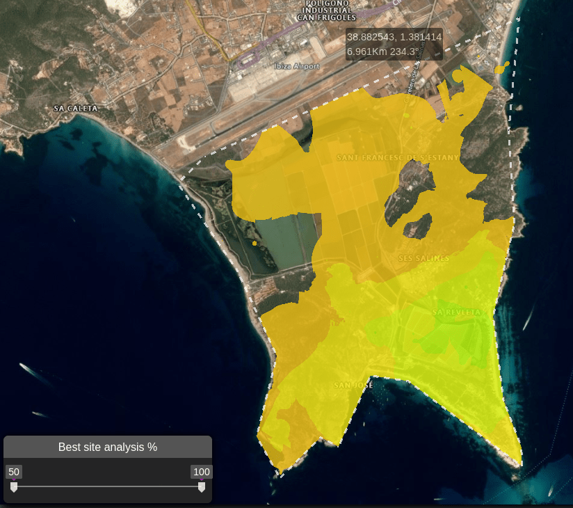
Best Site Analysis
If you select “Best Site Analysis” from the “Purpose” dropdown then this is used to upload a polygon of a boundary which is used with the best site analysis functionality. This is useful if you are working with very specific boundaries and don’t wish to keep redrawing the area. Instead you can upload your file and have the calculation repeated with the same values every time.
Upon successful upload of your boundary the best site analysis tool will be immediately fired off using your current settings.
For more information please consult the section relating to the best site analysis planning tool.
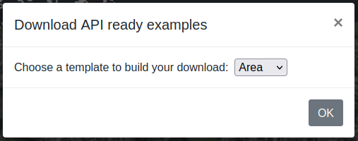
Automatic Processing Guidance
If you select “Automatic processing” from the “Purpose” dropdown then this will enable you to upload a simple CSV spreadsheet describing the sites in your network. This uses a subset of what is available in the API and all other settings will be set in your form at the point of upload eg. Radius and Resolution.
This is a simplified way to use the API via the user interface which has limited options compared to the full examples documented on GitHub
The CSV format must conform to one of two standards; a short format or a long format.
Short format CSV
Your CSV files must have these column headers:
NameLatitude: between -90 and 90 (required)Longitude: between -180 and 180 (required)Power_W: (required)Loss_dBAzimuth_deg: between 0 and 359Downtilt_deg: between 0 and 359Height_m: between 0.1 and 60000 (required)Gain_dB
Example CSV
Name,Latitude,Longitude,Power_dBm,Misc Loss (dB),Azimuth_deg,Downtilt_deg,Height_m,Gain_dB,Loss_dB
Site 1,38.9053686786203,1.42393869858255,30,0,240,10,6,8,1
Site 2,38.9071885546264,1.43414926725016,10,0,240,10,1,8,1
Site 3,38.9045598298649,1.43757317051595,1,0,240,10,10,8,1
Site 4,38.904250561729,1.43222332166316,2,0,240,10,11,8,1
Site 5,38.9072718158113,1.42824914822965,32,0,240,10,10,8,1
Site 6,38.9088894423094,1.43708404147798,43,0,240,10,9,8,1
Site 7,38.9113633880056,1.43029737607615,3,0,240,10,7,8,1
Site 8,38.9053686786203,1.43118392245747,44,0,240,10,8,8,1
Site 9,38.9068911924546,1.42500866835311,55,0,240,10,9,8,1
Site 10,38.9135993801199,1.43451611402864,77,0,240,10,7,8,1
Long format CSV
Your CSV files must have these column headers:
SiteLatitude: between -90 and 90 (required)Longitude: between -180 and 180 (required)Height_m(required)Frequency_MHz: between 2 and 100000(required)Bandwidth_MHz: between 0.1 and 200Power_W(required)Receiver_Height_m: between 0 and 60000Receiver_Gain_dBi: between -30 and 60Receiver_Sensitivity_dBmAntenna_Pattern: Pattern name or “Custom”Antenna_Polarisation: “V” for vertical or “H” for horizontalAntenna_Gain_dBiAntenna_Loss_dBAntenna_Azimuth_deg: between 0 and 359Antenna_Tilt_deg: between 0 and 359Antenna_Horizontal_Beamwidth_deg: between 0 and 360 (required for custom patterns)Antenna_Vertical_Beamwidth_deg: between 0 and 360 (required for custom patterns)Front_to_back: between 0 and 360 (required for custom patterns)Noise_floor_dBmMeasured_unitsColour_schemaModelContextDiffractionReliabilityProfile
Example CSV
Site,Latitude,Longitude,Height_m,Frequency_MHz,Bandwidth_MHz,Power_W,Antenna_Pattern,Antenna_Polarisation,Antenna_Loss_dB,Antenna_Azimuth_deg,Antenna_Tilt_deg,Antenna_Gain_dBi,Noise_floor_dBm,Model
Site 1,38.9053686786203,1.42393869858255,10,446,1.4,30,OEM Half-Wave Dipole,V,0,240,10,8,-120,Egli VHF/UHF (< 1.5GHz)
Site 2,38.9071885546264,1.43414926725016,11,800,10,10,OEM Half-Wave Dipole,V,10,240,10,8,-90,Egli VHF/UHF (< 1.5GHz)
Site 3,38.9045598298649,1.43757317051595,20,2400,20,1,OEM Half-Wave Dipole,H,11,240,10,8,-70,Egli VHF/UHF (< 1.5GHz)
Site 4,38.904250561729,1.43222332166316,15,2100,22,2,OEM Half-Wave Dipole,V,4,240,10,8,-180,Egli VHF/UHF (< 1.5GHz)
Site 5,38.9072718158113,1.42824914822965,7,900,1.9,32,OEM Half-Wave Dipole,H,5,240,10,8,-90,Egli VHF/UHF (< 1.5GHz)
Site 6,38.9088894423094,1.43708404147798,30,1700,1.8,43,OEM Half-Wave Dipole,V,6,240,10,8,-120,Egli VHF/UHF (< 1.5GHz)
Site 7,38.9113633880056,1.43029737607615,31,1800,18,3,OEM Half-Wave Dipole,H,1,240,10,8,-140,Egli VHF/UHF (< 1.5GHz)
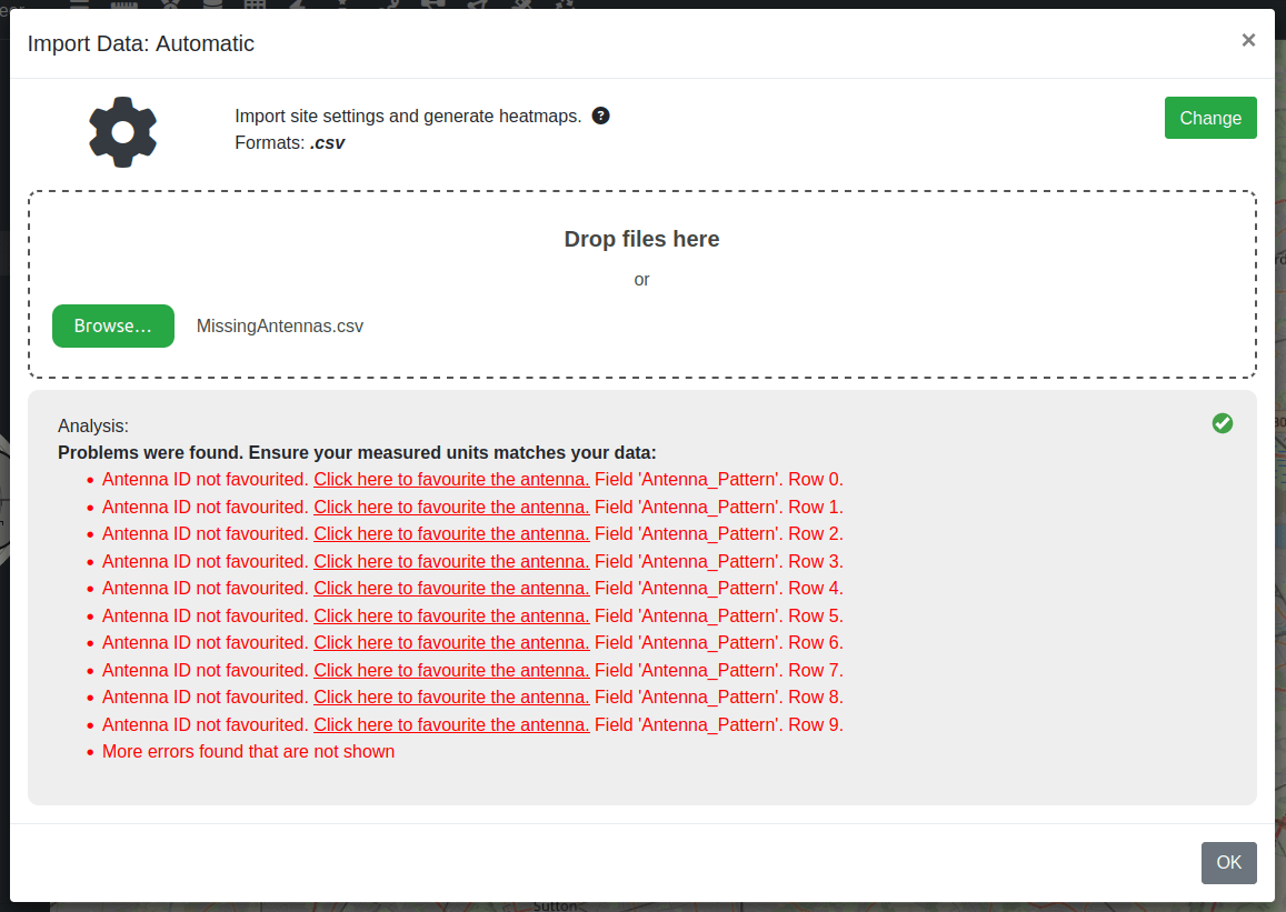
Troubleshooting - Missing Antenna
When specifying an antenna ID within your CSV for automatic processing, you should have the the antenna pattern favourited, otherwise you will be prompted with a validation error.
You can either follow the guide on favouriting antenna patterns, or during validation you can click on the prompt and the missing antenna patterns will be favourited, providing that they exist within the antennas database.
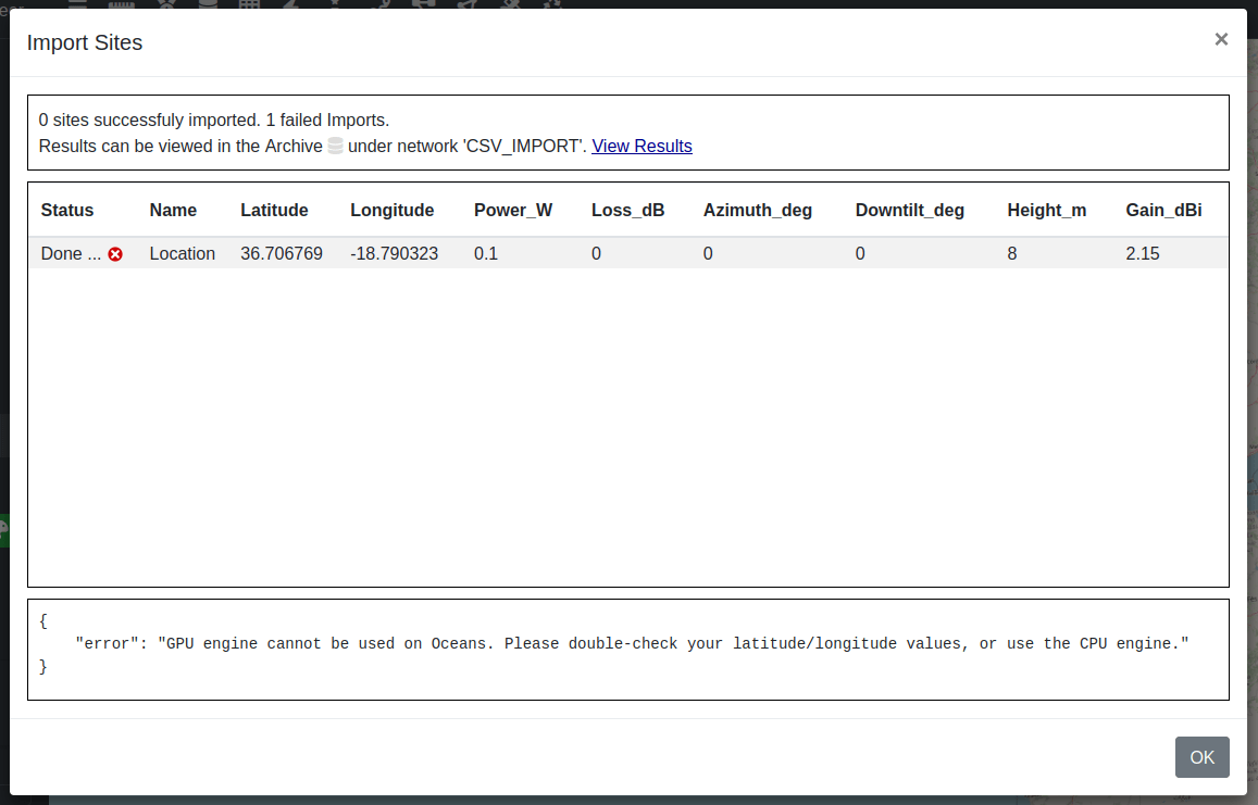
Troubleshooting - Calculation Response
If you wish to see the response for a calculation, you can click on the status icon for that calculation ( or
or  ).
).
After clicking on this a guidance box will be displayed at the bottom of the modal window. This can be useful for identifying why individual calculations have failed. Below shows an example.