


Common Tasks
The following are instructions for completing several common tasks in radio engineering. They are intended as a guide only. For detailed instructions on each component see the relevant documentation section.
Measure the coverage of a WISP tower
A WISP tower is going to be built and evidence is needed to justify the cost/benefit.
1. Create the tower coverage
Create the tower coverage as a layer using the interface. If the antenna pattern is known then use that for the most accurate model, otherwise you can use custom beamwidth values from the datasheet.
2. Upload zip code data for properties
Prepare a CSV spreadsheet for the area containing zip codes. These can be grouped by streets or neighbourhoods and the zip or address is the unique value in the id column.
Example property data
latitude |
longitude |
id |
group |
|---|---|---|---|
51.8668 |
-2.2066 |
GL43HX |
Barnwood |
51.8641 |
-2.2129 |
GL43HY |
Barnwood |
3. Download the results
You can download results as CSV by clicking the download button in the bottom left analysis window. This download will show you if a property is covered or not with a YES or NO. If your input data can be sorted and contains the same number of rows as the output, you can paste the YES/NO column into your input CSV for a very granular report into neighbourhood coverage.
Model multiple sites for multiple frequencies
The problem is how to efficiently model multiple locations but with different frequencies. The locations do not change.
1. Prepare a CSV spreadsheet
Instead of entering locations manually into the user interface, enter them into a CSV spreadsheet to eliminate error with (repeat) siting. The format should as a minimum contain the fields latitude and longitude:
latitude |
longitude |
|---|---|
51.8668 |
-2.2066 |
51.8641 |
-2.2129 |
2. Save radio settings as templates
Create your radio settings in the interface form and save them as a template. You will need a template for each frequency you need to test.
3. Import data
Select a template for the first frequency eg. Frequency1, then using the data import “MANET tool” option, load in the CSV. Each site will be modelled with the chosen frequency and associated settings. Repeat by loading the next template, and loading in the same CSV.
Design a network that meets a coverage requirement
The requirement is for 95% coverage of a city with a LPWAN smart meter network. The network must be economical yet provide good coverage. The consultant must be able to demonstrate planned coverage meets the requirement.
1. Prepare your data
The most important aspect of this task is to prepare your data. You need CSV spreadsheets for the properties or locations you would like covered (maximum 60,000 rows per spreadsheet in the interface) and another for the gateway locations (maximum 1000 rows in the interface).
Pay particular attention to the site name and network name fields as these will be needed later when finding, deleting or analysing the data.
Example property data
latitude |
longitude |
id |
group |
|---|---|---|---|
51.8668 |
-2.2066 |
CloudRF |
Barnwood |
51.8641 |
-2.2129 |
Roundabout |
Barnwood |
Example gateway data
This verbose format is for the user interface “site import” feature only. If you choose to use the API directly, you can use any format so long as it conforms to the API at the point of request. Examples are here: https://github.com/Cloud-RF/CloudRF-API-clients/tree/master/python
Site,Latitude (degrees),Longitude (degrees),Transmitter Height (m),Receiver Height (m),Receiver Gain (dBi),Receiver Sensitivity (dBm),Frequency (MHz),Bandwidth (MHz),RF Power (W),Antenna Pattern,Antenna Polarization,Antenna Loss (dB),Antenna Azimuth (degrees),Antenna Tilt (degrees),Antenna Gain (dBi),Noise floor (dBm),Model,Measured units,Context,Diffraction,Reliability,Profile,Colour schema,Antenna Horizontal Beamwidth (degrees),Antenna Vertical Beamwidth (degrees),Front to back
Site 1,38.9053686786203,1.42393869858255,10,10,8,-50,446,1.4,30,OEM Half-Wave Dipole,V,0,240,10,8,-120,Egli VHF/UHF (< 1.5GHz),Received Power (dBm),Average / Mixed,Knife edge,50% / -0dB (Optimistic),Minimal.clt,RAINBOW,1,1,8
Site 2,38.9071885546264,1.43414926725016,11,1,10,-60,800,10,10,OEM Half-Wave Dipole,V,10,240,10,8,-90,Egli VHF/UHF (< 1.5GHz),Received Power (dBm),Average / Mixed,Knife edge,50% / -0dB (Optimistic),Minimal.clt,RAINBOW,1,1,8
Site 3,38.9045598298649,1.43757317051595,20,5,5,-70,2400,20,1,OEM Half-Wave Dipole,H,11,240,10,8,-70,Egli VHF/UHF (< 1.5GHz),Received Power (dBm),Average / Mixed,Knife edge,50% / -0dB (Optimistic),Minimal.clt,RAINBOW,1,1,8
2. Process the gateway data
Using either an API client or the new “site import” functionality in the user interface, push the CSV data into the API with the “Area” API. This could be CPU or GPU powered and will create heatmaps in your account for analysis. If you have labelled the network properly it will be easy to find the data in your archive.
3. Load the data in the user interface
Load the layers on the map by either clicking their names from your archive or merging them into a super layer using the super layer utility. If you processed the data using the MANET API this is unncessary as the data is already a single layer.
4. Perform coverage analysis using the property data
Import the CSV data containing customer properties using the Coverage Analysis import option and expect to see coverage results displayed in the bottom left corner. Results will report coverage as a percentage so 90% would be covering 9/10 properties in an area.
5. Move or remove a gateway
If a gateway needs changing to meet the requirement (95%), remove it from the network by selecting and deleting it in the archive and then do it again at the new location.
6. Download results
You can download results as CSV by clicking the download button in the bottom left analysis window. This download will show you if a property is covered or not with a YES or NO. If your input data can be sorted and contains the same number of rows as the output, you can paste the YES/NO column into your input CSV for a very granular report into neighbourhood coverage.
Model HF NVIS coverage
Enter an appropriate frequency between 2 and 8MHz and a Tx power in watts.
Choose the HF NVIS model in the model menu. The antenna will be automatically set although you may choose the azimuth and gain. Use 0dBi if you are not sure of the gain or it is a whip. Set diffraction off to reveal any shadows although it will likely diffract into them given the frequency.
Choose the context/height to match the scenario. If it’s day time then the D layer will be present but will attenuate low frequencies so bear this in mind. If it’s night time, use the F layer. If there’s uncertainty then use the E layer for a compromise.
For the receiver use 0dBi for a whip antenna.
Use the CPU engine with 180m resolution for links out to 200km. Otherwise use the GPU engine.
Click the map or press play or change a value like azimuth to trigger a calculation.
Find the best HF frequency for a month
Choose the HF Skywave model in the model menu
Choose the month and hour
Set the sunspot number to match latest data (100 if unsure)
Use the path tool to click on the distant station on the map. The link chart will display showing the best frequencies to use for the link and time. If the chart is blank, there is nothing to show above 0dB SNR so you should consider your antenna, antenna height and power.
Model HF Skywave coverage
From the “Model” menu select “HF Skywave”. This uses the VOACAP engine.
At the “Site/Tx” menu set your antenna height above the ground, e.g. 6m.
At the “Signal” menu set your frequency and RF power. Default values of 10MHz and 30W will be set.
At the “Antenna” menu, choose your pattern and appropriate gain, e.g. Horizontal Dipole, 2dBi.
At the “Mobile/Rx” menu set the threshold to -121dBm which is an S1 signal.
In the “Output” menu choose the HF S1-S9 colour schema.
Set the radius to reach your distant station eg. 2000km.
Click the green play button to model the HF area coverage.
If coverage is not showing, check youy are using the HF colour key and your receiver threshold is at least -120dBm.
We have a series on videos for HF modelling on our YouTube Channel.
Model a flight path
Prepare your flight path as a KML linestring. These files can be exported from adsb exchange.
Open the import dialog and choose “route analysis”. Load in the KMZ/KMZ.
The points should display on the map if a valid linestring was found.
Place and configure your ground station and click calculate to observe coverage along the flight path. If different altitudes are detected, the option to model a ground overlay will be removed so you only get coloured balls floating above the ground.
Test a route for coverage against a network
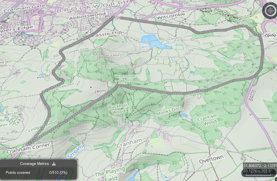
Create your route as a KML linestring in a suitable application, such as Google Earth or equivalent. Save it as KML or KMZ.
Import the KML/KMZ file using the file import dialog as “Coverage analysis”. Lots of grey points will be added to the map.
Create or reload a heatmap layer to test for coverage. The coverage will be reported in the coverage analysis dialog in the bottom left corner.
For a MANET network, enable the MANET tool and ensure heatmaps are enabled by clicking the donut icon in the MANET dialog. Links are ignored here. Place the MANET nodes by clicking upon the map.
Note that the settings for each node can be different but can only be defined prior to placing the node. Once placed, a node’s frequency and power cannot be changed but you can change global network values such as environmental settings.
See the Web Interface Import Data > Coverage Analysis section for more detail on this topic