Summary
We field tested our software to improve it for beyond line of sight planning. From analysis of data we have improved diffraction accuracy, clutter profiles and crucially have proven that high resolution LiDAR is not the best choice for beyond line of sight or sub GHz modelling. An RMSE modelling error of 5.2dB was achieved as a result.
Modelling can only be as accurate as the inputs.
Given accurate reference data and accurate RF parameters it can be very accurate but achieving both conditions requires careful and delicate calibration of dozens of variables. Thankfully this time intensive process is only necessary when changing hardware which for most organisations is a cycle measured in years.
The reference data used could be a digital terrain model like SRTM, a digital surface model like ALOS30, high fidelity LiDAR or landcover like ESA Worldcover. As we demonstrate, high resolution does not always translate to high accuracy in beyond line of sight RF.
LiDAR is great, but it’s not a silver bullet
You can have the most expensive 50cm LiDAR money can buy and still not achieve real world accuracy or a notable gain over 1m or 2m data (unless you’re planning for a model village). LiDAR on its own cannot model beyond line of sight, essential for sub GHz planning, which is a risk we’ll explore when planning tool design is focused on sales and marketing, not actual RF Engineering.
Controversially, you can get better BLOS modelling accuracy with basic terrain data enhanced with calibrated clutter profiles which we’ll demonstrate below.
The best data to use depends on the technology and requirements. LiDAR is unbeatable for line of sight planning, but won’t help you in the woods, or beyond line of sight without a proper physics propagation engine.
Unless your network is composed of static masts eg. Fixed wireless access (FWA), then chances are you are working non line of sight between radios so LiDAR should be used carefully.
“Line of sight” field testing Feb 2022
Last year we field tested LTE 800MHz in the Peak district and achieved excellent calibration figures for distant hilltop towers looking onto open moorland. This was predictable given the legacy cellular models we used were developed from similar measurements. As the blog described, the harder calibration was inside a wood where the LiDAR data proved unsuitable. Due to the simplistic nature of first return LiDAR, a tree canopy appears as a solid immutable obstacle. You can model the RF as it hits the tree canopy but not where it matters, on the ground inside the trees. This key finding accelerated and matured our developments with tooling to support calibration with survey data in CSV format and user configurable environment profiles.

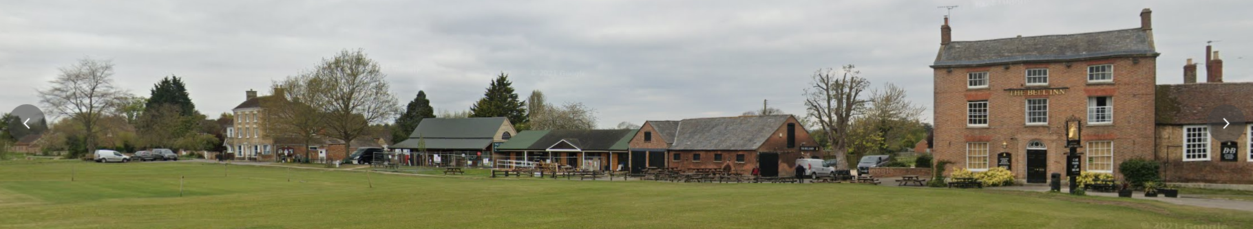
“Non Line of sight” field testing, Feb 2023
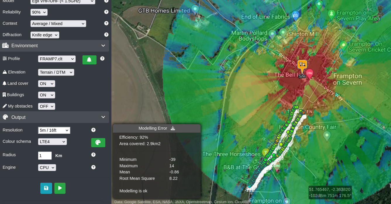
This year we field tested LTE 800MHz again but this time in a old Gloucestershire village, Frampton on Severn, where the tower was deliberately obstructed and the solid stone buildings in the village meant we were measuring diffraction, coming from rooftops of single, double and triple storey buildings. The test data was collected from 2 handheld LTE test devices using a combination of Network Signal Guru (NSG) and CellMapper for Android. This app reports signal values and logs cell metadata with locations to a CSV file which we can analyse.
Some variables were unknown such as RF power, which required us to take measurements on the green in full line of sight. These “power readings” allowed us to reverse engineer the cell power as approximately 40dBm (10W) which would be appropriate for a cell serving a village.
Received Signal Received Power (RSRP)
The measured power value is Received Signal Received Power (RSRP) which is a LTE dBm value determined by the bandwidth, in this case 10MHz like most LTE Band 20 signals in Europe.
RSRP is lower than the carrier signal (Received Power) which is agnostic to bandwidth, but also measured in dBm.
Be careful not to confuse the two units of measurement as they can vary by more than 27dB!! A carrier signal of -80dBm might have a RSRP of -108dBm or lower depending on bandwidth. RSRP is usable down to -120dBm.
| Received power dBm | Bandwidth MHz | RSRP dBm |
|---|---|---|
| -70 | 10 | -97.8 |
| -80 | 10 | -107.8 |
| -90 | 10 | -117.8 |
Diffraction
Diffraction is the effect that occurs when radiation hits an edge like a rooftop or a hilltop. The wavefront radiates from that edge with resulting power determined by several factors like height and wavelength. Much like a game of pool, the angle of incidence determines the angle of reflection so a tall building will cast a long RF shadow before the diffracted signal is available again beyond the shadow. A proper diffraction shadow has soft edges as the RF scatters in all directions. LiDAR data creates sharp shadows, even when trees have no leaves.
The CloudRF service has two diffraction capable CPU and GPU engines which use a proprietary algorithm based upon Huygen’s formula which considers obstacle dimensions and wavelength.

Which propagation model is best for 800MHz?
Most propagation model curves follow similar trajectories but differ by only a modest amount of dB in relation to the impact of an obstacle. The choice of model is therefore less important, in our experience, than getting the obstacle data right so for a cellular base station, you could choose to calibrate against any empirical or deterministic model which supports that frequency. Each model has a reliability margin to help align and tune it. For UHF the advanced (and default) ITM model is preferable as it was designed for NLOS broadcasting with complex diffraction routines. For this test we picked the simpler Egli VHF/UHF model with basic knife edge diffraction since this features in both our CPU and GPU engines, and we want to calibrate both.

What is “accurate”?
The cellular modem used to record power levels has a measurement error of -/+ 3dB so any reading cannot be more accurate than this. Therefore, if calibration of field measurements returns a Root Mean Square (RMSE) value of 8dB, this can be considered to be composed of measurement error and (5dB of) modelling error.
For Line of sight, a modelling error level of < 10dB is ok, < 5dB is good, and < 3dB is excellent. This is the easy part which for some basic tools is enough.
For non line of sight (which covers much more complex scenarios), the error doubles so an error level of < 20dB is ok, < 10dB is good and < 6dB is excellent.
For our field testing, we achieved a non line of sight calibration with 5.2dB of modelling error which we were content with. We are confident we can improve upon this with richer clutter data which we are developing presently.
Results
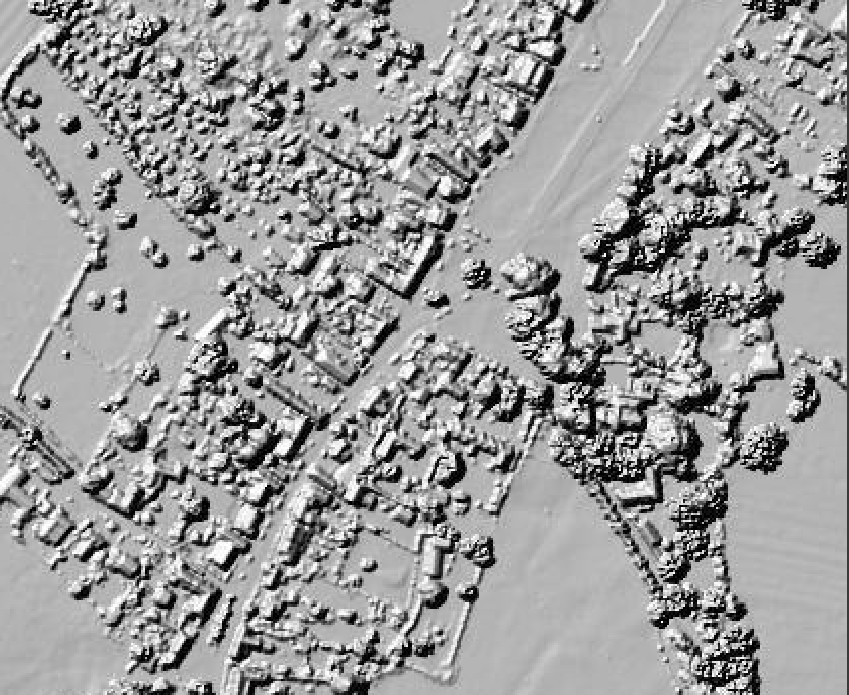
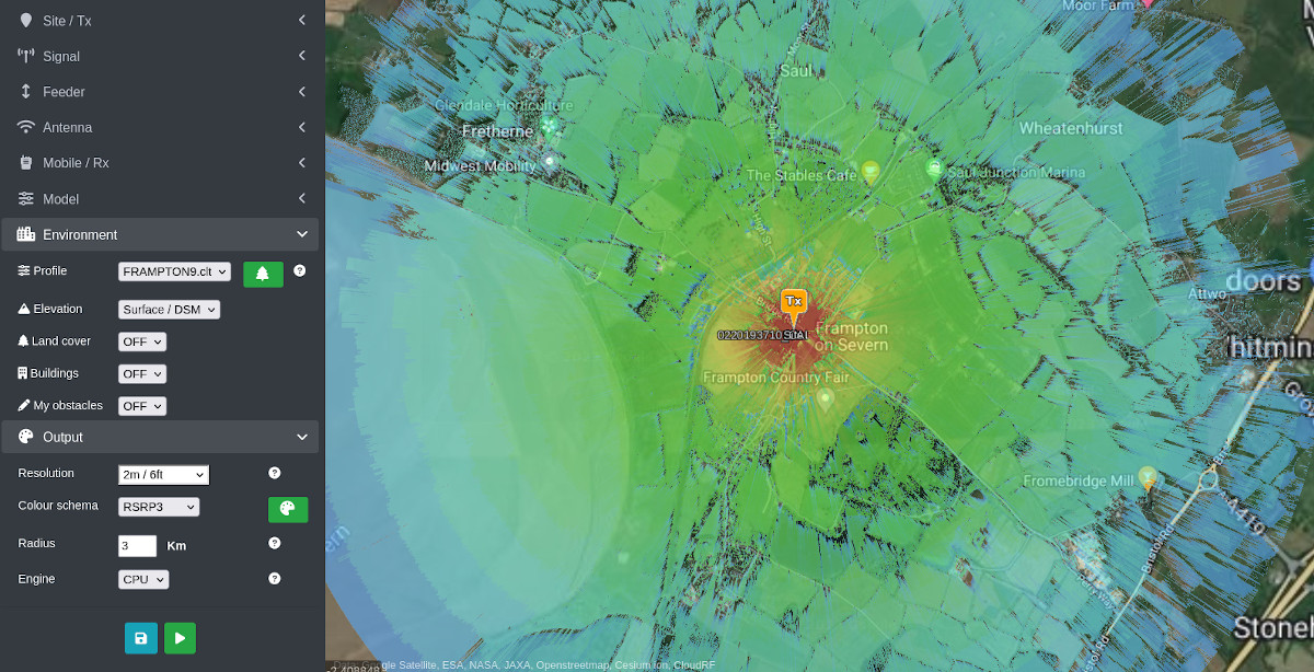
1m LiDAR – It isn’t as useful as it looks
Using 1m LiDAR for the village we generated a sharp heatmap sensitive to chimney stacks and even parked vehicles which made for a very crisp result visually but the first-pass correlation with the field measurements showed it was conservative, which arguably is a safe default if you’re unsure.
The reason was a combination of trees and buildings. The village had trees on the green but due to the season, none were in leaf so signals would travel through them with relatively reduced attenuation. The LiDAR data however, regards a tree as a solid obstacle so results in an overly conservative prediction for measurements beyond the trees. Attenuation through buildings is a weakness of LiDAR in 2.5D RF modelling using this raster data.
You can show RF on the roof and if diffraction is calibrated, beyond the diffraction shadow as the signal hits the ground but not within the shadow itself where through-building signals reside.

The LiDAR result was improved with positive adjustments to the diffraction routine in SLEIPNIR, our CPU engine. As a result, diffraction is slightly more optimistic and the correlation with field measurements was improved.
The best LiDAR score, subtracting 3dB of receiver error was a modelling RMSE of 7.28dB.
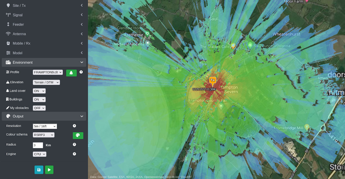
DTM and Landcover – Better than LiDAR?
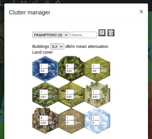
Using 30m DTM with layered 10m Landcover and 2m buildings, sampled at 5m resolution, higher calibration was achieved despite the loss of resolution. The reason is the Landcover offers through-material attenuation which can be adjusted to match field measurements. In this case, the “trees” and “urban” height and attenuation values were manipulated until coverage matched the results with high accuracy.
The best Landcover score, subtracting 3dB of receiver error was a modelling RMSE of 5.22dB.
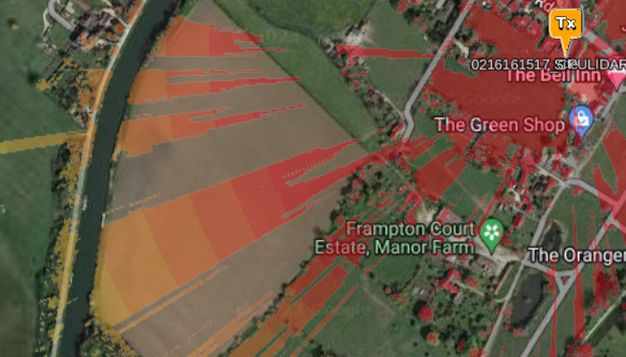
A / B comparison – LiDAR and Landcover
Using our calibrated settings, we extrapolated coverage out to 3km radius to model the whole cell. Here you can clearly see differences in coverage between the two data sets. With LiDAR, coverage is bouncing off hard tree canopies and casting sharp shadows on obstacles like hedgerows. With Landcover, we still have diffraction but more attenuation from obstacles which creates major nulls and also softer diffraction shadows, set by our clutter profile.
A look forward
Findings from this field testing will be worked back into the CloudRF service in coming days, followed by SOOTHSAYER in due course, as new releases for our SLEIPNIR CPU engine, GPU engine and better default clutter values. We are developing sharper, and economically viable, global clutter data to improve on these scores, but won’t say how just yet 😉
