“I’ve never seen modelling that matches the real world”
Anon
Noise in the RF spectrum is a growing issue. It undermines the performance of systems and requires careful spectrum management and deconfliction to mitigate its impact. Sources of noise can be natural, industrial or man made. Regardless of the source, or intent, the issue needs understanding and dealing with to operate effectively in congested spectrum.
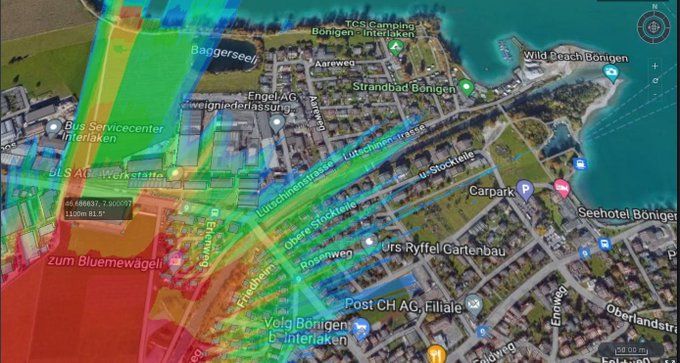
Radio users working in cities know about this problem all too well. They can describe the symptoms but are unable to visualise the full impact, and in doing so realise a solution such as an adjustment, through a lack of tooling. Many organisations have bought receivers for use at the edge, and back office software for planning but the two rarely meet…
Noise floor and SNR
The noise floor describes the average minimum RF power in the spectrum. There are different ways to measure it, and depending on the requirement you may want the peak power but for our purposes we are using the mean dBm value within the channel. A quiet noise floor value is -120dBm, subject to bandwidth. The higher this value, the less range you are communicating.
Signal to Noise Ratio (SNR), measured in dB, describes a signals power above the noise. A good signal might be 20dB above the noise and a weak signal only 3dB. Different signals have different SNR requirements; GPS for example uses a BPSK signal with a very low 2dB requirement so it’s barely visible in the noise whereas a DVB QAM signal needs a prominent 20dB SNR to deliver an error free video signal.
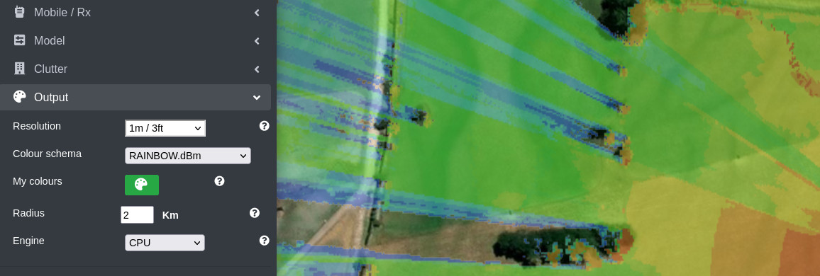
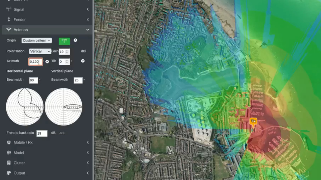
In CloudRF, both noise and SNR can be defined to simulate different environments and different waveforms.
A good guess – Johnson-Nyquist noise
Without the presence of man made signals, the RF spectrum has a natural noise floor called the thermal noise floor. This can be calculated with temperature (noise increases with temperature) and bandwidth (More bandwidth equals more noise).
Noise dBm = -173.8 + 10 log10(Frequency in Hertz)
Calculators exist to compute this value based on the Johnson-Nyquist formula. We use this in our interface so when you change bandwidth the noise floor is set. This is a good start, consider it a 75% guess, but is not the real noise. To get that you need to go to that place and measure it.
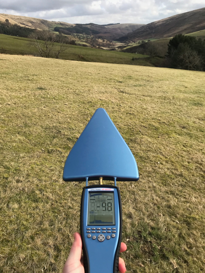
Measuring noise with an RFeye Node
To measure the noise floor accurately you need a high quality receiver. Low quality SDR receivers are easy to come by but will not be able to give you a more accurate noise value than the previously mentioned bandwidth formula.
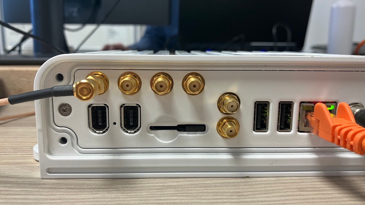
The CRFS RFeye Node is a high performance RF receiver with an excellent dynamic range, industry leading low noise figure, and sensitivity. The API enabled receiver is in use worldwide for remote spectrum monitoring making it an ideal candidate for integration, especially since it has open source client scripts!
Integration with the CloudRF API
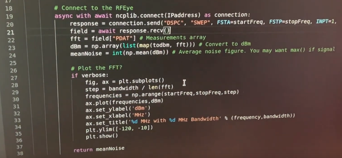
We imported the NCP client library into our open source API client so we could query the noise for our target frequency and bandwidth. Every time our script processes a site, the noise is tested and the result spliced into our site request.
In return we get a model which uses a real noise floor value. Typically this is higher than the formula method resulting in reduced coverage.
The beauty of this integration is the receiver can be in another county but the modelling can be conducted with high precision from home. With the scalability of the API it unlocks several possibilities:
Model a spreadsheet for a large network, and sample noise floor from local receivers instead of using a generic best guess value
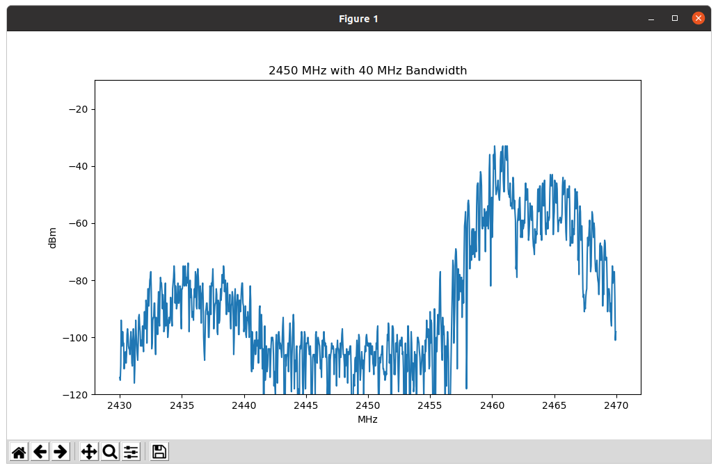
Model a route for a drone with different noise values along the route. If you’ve ever lost communications with a distant 2.4GHz drone that had LOS this was likely WiFi noise
Model a radio and/or a waveforms performance in a remote location without visiting or deploying equipment which is expensive and time consuming
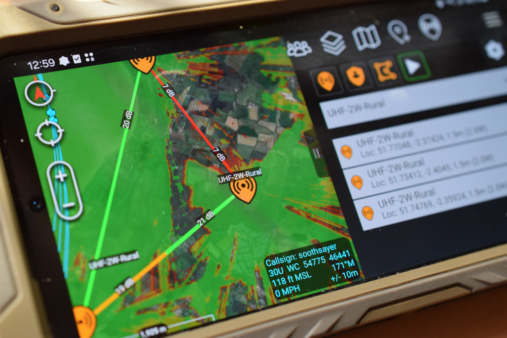
Demo video
In this video we put it all together to incorporate live noise into our modelling. We’re executing one site at a time, but with a spreadsheet, the API client will automatically process a network of sites.
Dynamic noise floor modelling with a CRFS RFeye receiver
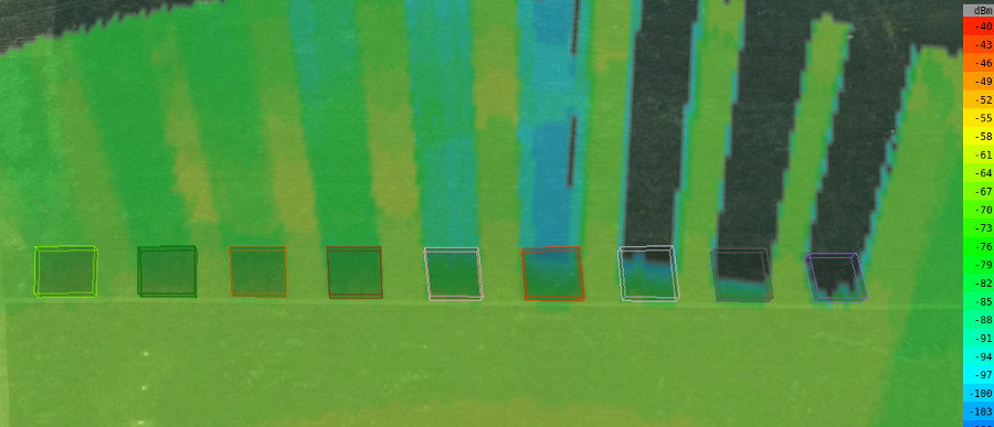
We field tested our software to improve it for beyond line of sight planning. From analysis of data we have improved diffraction accuracy, clutter profiles and crucially have proven that high resolution LiDAR is not the best choice for beyond line of sight or sub GHz modelling. An RMSE modelling error of 5.2dB was achieved as a result.
Modelling can only be as accurate as the inputs.
Given accurate reference data and accurate RF parameters it can be very accurate but achieving both conditions requires careful and delicate calibration of dozens of variables. Thankfully this time intensive process is only necessary when changing hardware which for most organisations is a cycle measured in years.
The reference data used could be a digital terrain model like SRTM, a digital surface model like ALOS30, high fidelity LiDAR or landcover like ESA Worldcover. As we demonstrate, high resolution does not always translate to high accuracy in beyond line of sight RF.
Calibrating modelling with LiDAR data to match field measurements
LiDAR is great, but it’s not a silver bullet
You can have the most expensive 50cm LiDAR money can buy and still not achieve real world accuracy or a notable gain over 1m or 2m data (unless you’re planning for a model village). LiDAR on its own cannot model beyond line of sight, essential for sub GHz planning, which is a risk we’ll explore when planning tool design is focused on sales and marketing, not actual RF Engineering.
Controversially, you can get better BLOS modelling accuracy with basic terrain data enhanced with calibrated clutter profiles which we’ll demonstrate below.
The best data to use depends on the technology and requirements. LiDAR is unbeatable for line of sight planning, but won’t help you in the woods, or beyond line of sight without a proper physics propagation engine.
Unless your network is composed of static masts eg. Fixed wireless access (FWA), then chances are you are working non line of sight between radios so LiDAR should be used carefully.
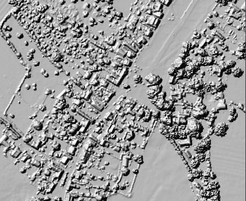
Public 1m LiDAR data showing cars, trees and houses
“Line of sight” field testing Feb 2022
Last year we field tested LTE 800MHz in the Peak district and achieved excellent calibration figures for distant hilltop towers looking onto open moorland. This was predictable given the legacy cellular models we used were developed from similar measurements. As the blog described, the harder calibration was inside a wood where the LiDAR data proved unsuitable. Due to the simplistic nature of first return LiDAR, a tree canopy appears as a solid immutable obstacle. You can model the RF as it hits the tree canopy but not where it matters, on the ground inside the trees. This key finding accelerated and matured our developments with tooling to support calibration with survey data in CSV format and user configurable environment profiles.
CSV import utility – developed for analysing field test data
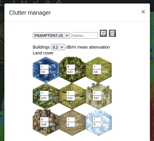
Clutter manager
“Non Line of sight” field testing, Feb 2023
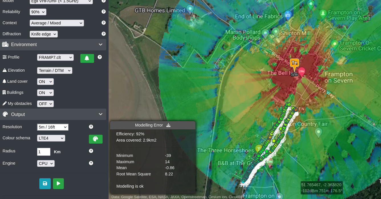
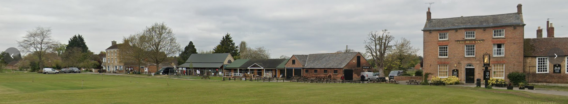
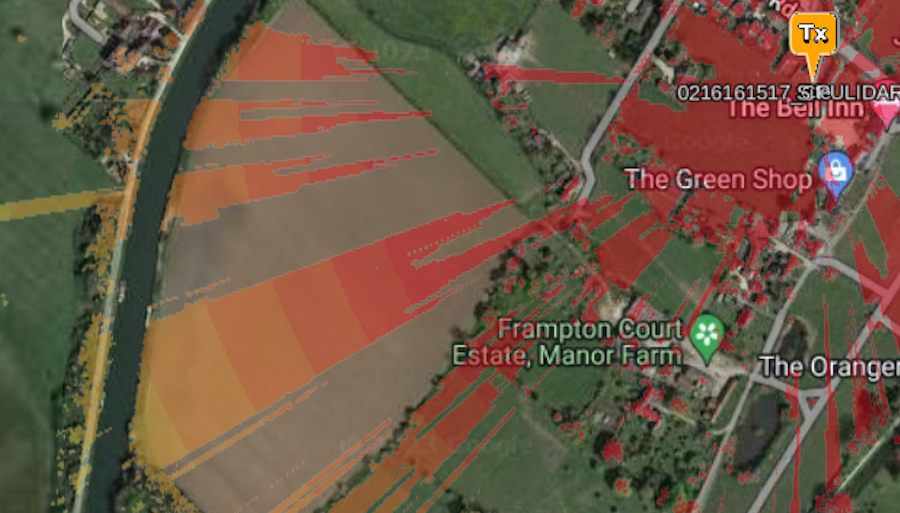
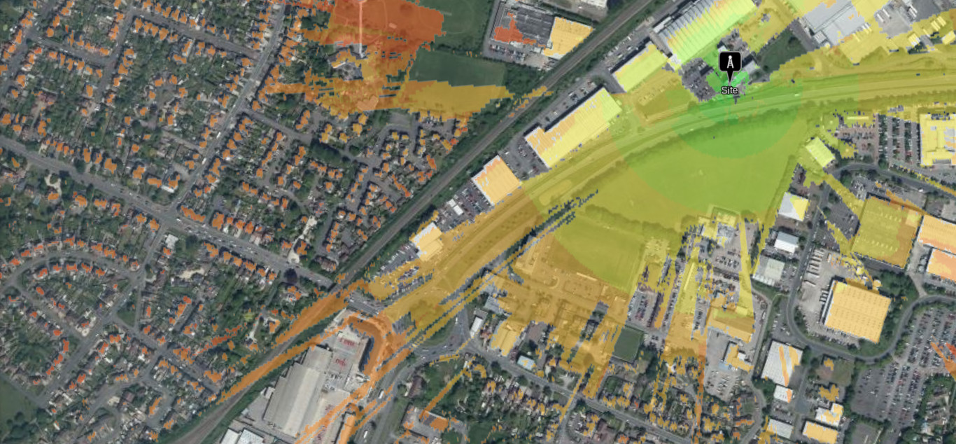
This year we field tested LTE 800MHz again but this time in a old Gloucestershire village, Frampton on Severn, where the tower was deliberately obstructed and the solid stone buildings in the village meant we were measuring diffraction, coming from rooftops of single, double and triple storey buildings. The test data was collected from 2 handheld LTE test devices using a combination of Network Signal Guru (NSG) and CellMapper for Android. This app reports signal values and logs cell metadata with locations to a CSV file which we can analyse.
Some variables were unknown such as RF power, which required us to take measurements on the green in full line of sight. These “power readings” allowed us to reverse engineer the cell power as approximately 40dBm (10W) which would be appropriate for a cell serving a village.
Frampton on Severn. The cell tower is to the far right behind the pub.
Received Signal Received Power (RSRP)
The measured power value is Received Signal Received Power (RSRP) which is a LTE dBm value determined by the bandwidth, in this case 10MHz like most LTE Band 20 signals in Europe.
RSRP is lower than the carrier signal (Received Power) which is agnostic to bandwidth, but also measured in dBm.
Be careful not to confuse the two units of measurement as they can vary by more than 27dB!! A carrier signal of -80dBm might have a RSRP of -108dBm or lower depending on bandwidth. RSRP is usable down to -120dBm.
Received power dBm
Bandwidth MHz
RSRP dBm
-70
10
-97.8
-80
10
-107.8
-90
10
-117.8
Relationship between power, bandwidth and RSRP at 10MHz
Diffraction
Diffraction is the effect that occurs when radiation hits an edge like a rooftop or a hilltop. The wavefront radiates from that edge with resulting power determined by several factors like height and wavelength. Much like a game of pool, the angle of incidence determines the angle of reflection so a tall building will cast a long RF shadow before the diffracted signal is available again beyond the shadow. A proper diffraction shadow has soft edges as the RF scatters in all directions. LiDAR data creates sharp shadows, even when trees have no leaves.
The CloudRF service has two diffraction capable CPU and GPU engines which use a proprietary algorithm based upon Huygen’s formula which considers obstacle dimensions and wavelength.
Exaggerated diffraction caused by solid LiDAR
Which propagation model is best for 800MHz?
Most propagation model curves follow similar trajectories but differ by only a modest amount of dB in relation to the impact of an obstacle. The choice of model is therefore less important, in our experience, than getting the obstacle data right so for a cellular base station, you could choose to calibrate against any empirical or deterministic model which supports that frequency. Each model has a reliability margin to help align and tune it. For UHF the advanced (and default) ITM model is preferable as it was designed for NLOS broadcasting with complex diffraction routines. For this test we picked the simpler Egli VHF/UHF model with basic knife edge diffraction since this features in both our CPU and GPU engines, and we want to calibrate both.
Path loss curves for propagation models
What is “accurate”?
The cellular modem used to record power levels has a measurement error of -/+ 3dB so any reading cannot be more accurate than this. Therefore, if calibration of field measurements returns a Root Mean Square (RMSE) value of 8dB, this can be considered to be composed of measurement error and (5dB of) modelling error.
For Line of sight, a modelling error level of < 10dB is ok, < 5dB is good, and < 3dB is excellent. This is the easy part which for some basic tools is enough.
Line of Sight coverage: Good for above UHF only
For non line of sight (which covers much more complex scenarios), the error doubles so an error level of < 20dB is ok, < 10dB is good and < 6dB is excellent.
For our field testing, we achieved a non line of sight calibration with 5.2dB of modelling error which we were content with. We are confident we can improve upon this with richer clutter data which we are developing presently.
Results
1m LiDAR – It isn’t as useful as it looks
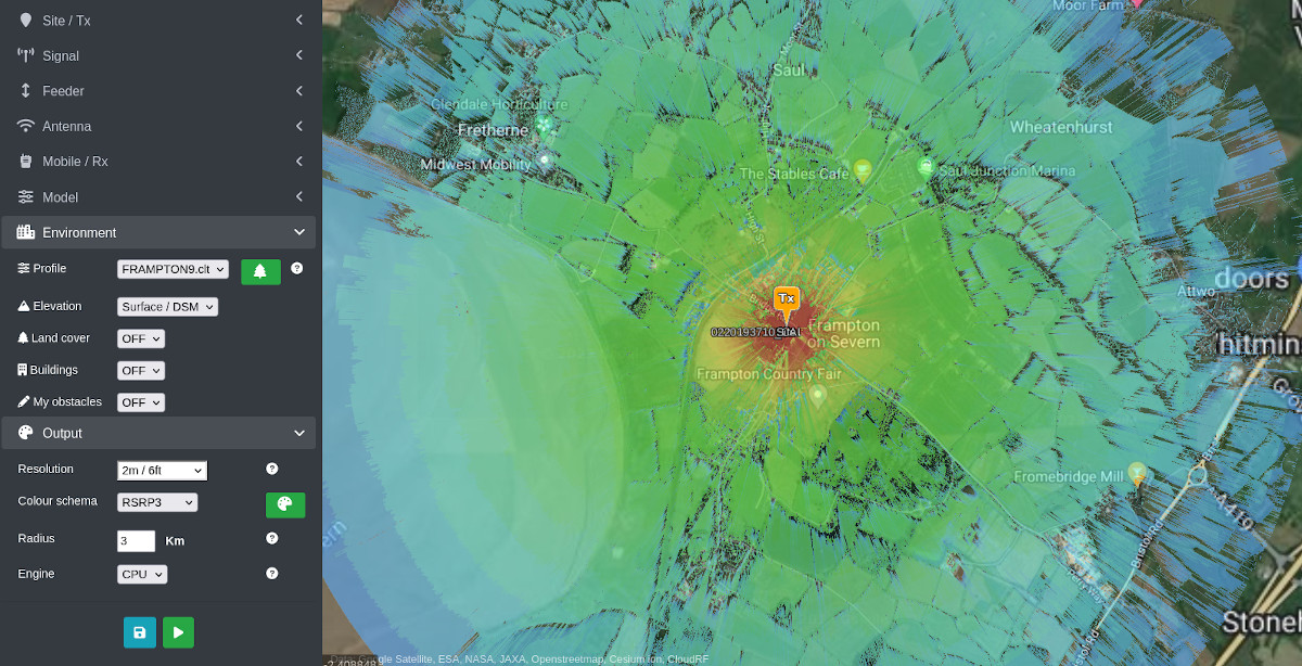
Using 1m LiDAR for the village we generated a sharp heatmap sensitive to chimney stacks and even parked vehicles which made for a very crisp result visually but the first-pass correlation with the field measurements showed it was conservative, which arguably is a safe default if you’re unsure.
The reason was a combination of trees and buildings. The village had trees on the green but due to the season, none were in leaf so signals would travel through them with relatively reduced attenuation. The LiDAR data however, regards a tree as a solid obstacle so results in an overly conservative prediction for measurements beyond the trees. Attenuation through buildings is a weakness of LiDAR in 2.5D RF modelling using this raster data.
You can show RF on the roof and if diffraction is calibrated, beyond the diffraction shadow as the signal hits the ground but not within the shadow itself where through-building signals reside.
LiDAR calibration showing a mean error of -1dB and a total RMSE error of 10dB.
The LiDAR result was improved with positive adjustments to the diffraction routine in SLEIPNIR, our CPU engine. As a result, diffraction is slightly more optimistic and the correlation with field measurements was improved.
The best LiDAR score, subtracting 3dB of receiver error was a modelling RMSE of 7.28dB.
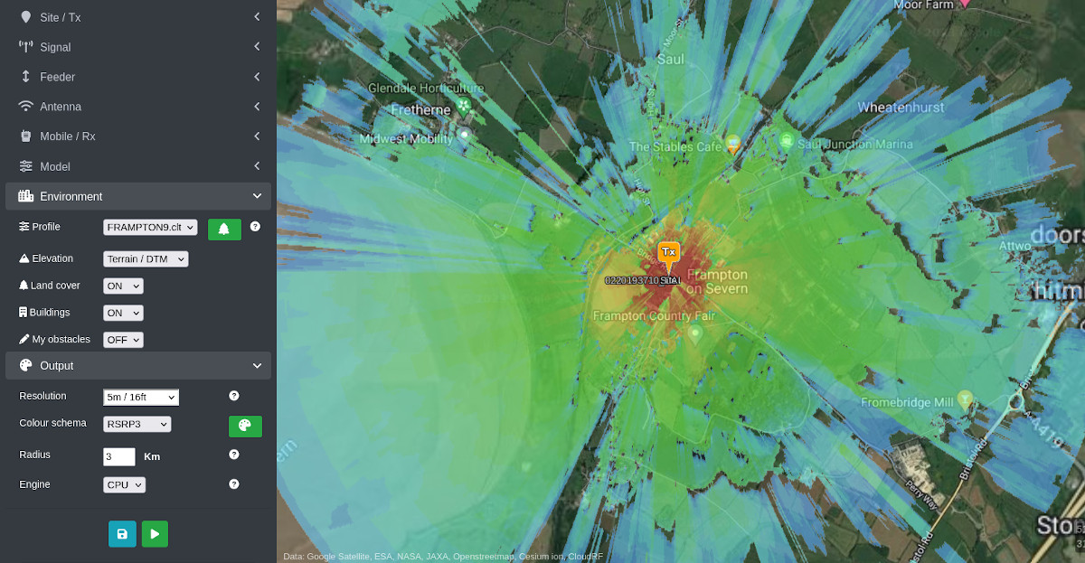
DTM and Landcover – Better than LiDAR?
Using 30m DTM with layered 10m Landcover and 2m buildings, sampled at 5m resolution, higher calibration was achieved despite the loss of resolution. The reason is the Landcover offers through-material attenuation which can be adjusted to match field measurements. In this case, the “trees” and “urban” height and attenuation values were manipulated until coverage matched the results with high accuracy.
The best Landcover score, subtracting 3dB of receiver error was a modelling RMSE of 5.22dB.
Landcover calibration produced a better result – without breaking the bank
A / B comparison – LiDAR and Landcover
Using our calibrated settings, we extrapolated coverage out to 3km radius to model the whole cell. Here you can clearly see differences in coverage between the two data sets. With LiDAR, coverage is bouncing off hard tree canopies and casting sharp shadows on obstacles like hedgerows. With Landcover, we still have diffraction but more attenuation from obstacles which creates major nulls and also softer diffraction shadows, set by our clutter profile.
Lidar coverageLandcover coverage
A look forward
Findings from this field testing will be worked back into the CloudRF service in coming days, followed by SOOTHSAYER in due course, as new releases for our SLEIPNIR CPU engine, GPU engine and better default clutter values. We are developing sharper, and economically viable, global clutter data to improve on these scores, but won’t say how just yet 😉
Today we have launched a new GPU accelerated API called “Multisite” which is capable of modelling hundreds of sites in the time we previously would have done one. This exponential increase in capability grew from our Best Site Analysis (BSA) capability which uses a Monte Carlo technique to test hundreds of random locations, and from the intermediate outputs, reduce them to reveal the optimal location(s) for radio communication.
The difference in Multisite is that the locations are not random, they are defined by the client.
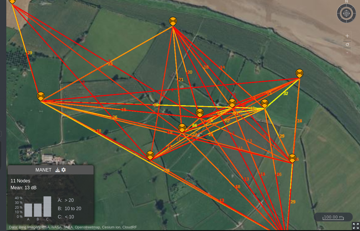
A link is not coverage
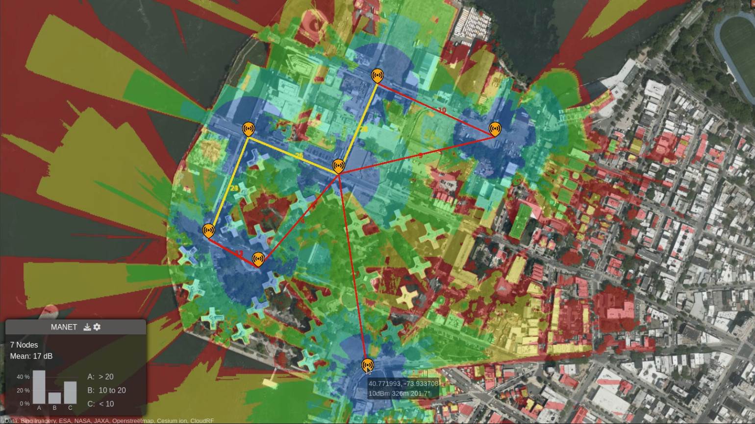
Following customer feedback on our MANET planning tool which up until now created point-to-point links between nodes we investigated the feasibility of showing all the coverage, or in classic modelling terminology a point-to-multipoint aka a heatmap.
The reason this is important in MANET planning is you need to see the whole network coverage to understand where you are serving and where your gaps are. Links won’t show you coverage gaps unless it involves the node location so you will find out about these when it’s too late. Links are useful for seeing a network’s geometry and overall health but are of limited use for tactical RF planning where the network members are expected to be agile.
A bonus feature is that a heatmap scales better than links which get very cluttered in an interface when many overlap. A heatmap is much easier for a human to digest than a game of radio kerplunk which can overload an operator.
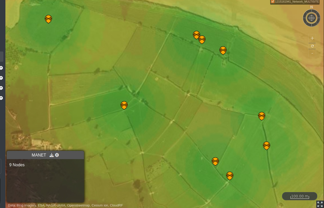
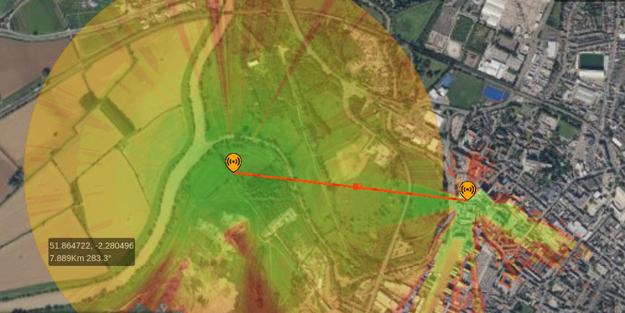
MANET linksLinks with a heatmapHeatmap onlyA link between two very different sites
Faster, cleaner more scalable MANET planning
As this is GPU powered it is faster than the previous CPU powered link calculations. By removing the links, the view is less cluttered for busy networks and this can scale to a significant number of nodes in a single request.
During testing we were modelling 100 nodes in under 2 seconds, which includes communication latency to a production server in Europe. We achieved 3.1 seconds for 200 nodes at 10m resolution with 1km radius each and are confident we can do 500 nodes, like BSA does, and reduce the time further with infrastructure adjustments and a local server. Most of the delay is in data preparation and post processing, the actual computation is milliseconds so real-time modelling for multiple fast moving tracks is viable.
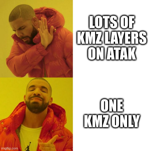
The heatmap exists in your archive as a standard layer so can be exported to KMZ, KML, GeoTIFF, SHP, URL or HTML via the normal archive functions.
Urban demo, NYC
In this early demo, MANET nodes are manually placed and adjusted. The coverage heatmap and links automatically update as nodes are added, removed or moved.
Multisite demo with MANET radios in a Urban environment
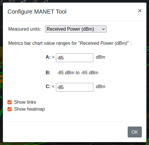
How do I enable the heatmap?
If you have a Gold account, open the MANET planning tool from the top bar then click the cog on the MANET window which appears. In the tools options, you can select either links, heatmap or both.
MANET tool options
Documentation
The capability is available in API and UI version 3.7.
This restriction does not apply to the MANET links and the points API which that uses.
Developer’s guide
A multisite request uses the same JSON structure and values as a area request only instead of a single transmitter object, it has an array of transmitters with no upper limit.
Each transmitter can have a different antenna so you could define several omni directional nodes with a single distant directional node, a common MANET design.
In this example, two MANET radios with 20MHz bandwidth in SNR mode are modelled together. The transmitters differ in location and power but the receiver, environment, model and output sections and common.
Now that we’ve published the API, the fun part of making interfaces for it has already started. The first of which is the enhancement to the MANET planning tool. Expect to see more interfaces and demos, at scale, shortly covering moving vehicles, large networks and ATAK integration where we plan to redefine the meaning of “radio check” with a whole network coverage map.
If you are an integrator or developer of a map and are interested in incorporating this unique layer, get in touch and save yourself years of R&D. White labeling options available.
Here’s a roundup of what’s changed since June. As always it’s been a busy period of development which we’ve matched with a focus on maintenance and bugfixes. Our backlog of feature and change requests stands at 28 for the UI and 23 for the API with all priority issues resolved.
The deck is now clear for a dynamic network planning feature which will be integrated in December.
UI changes, June to November
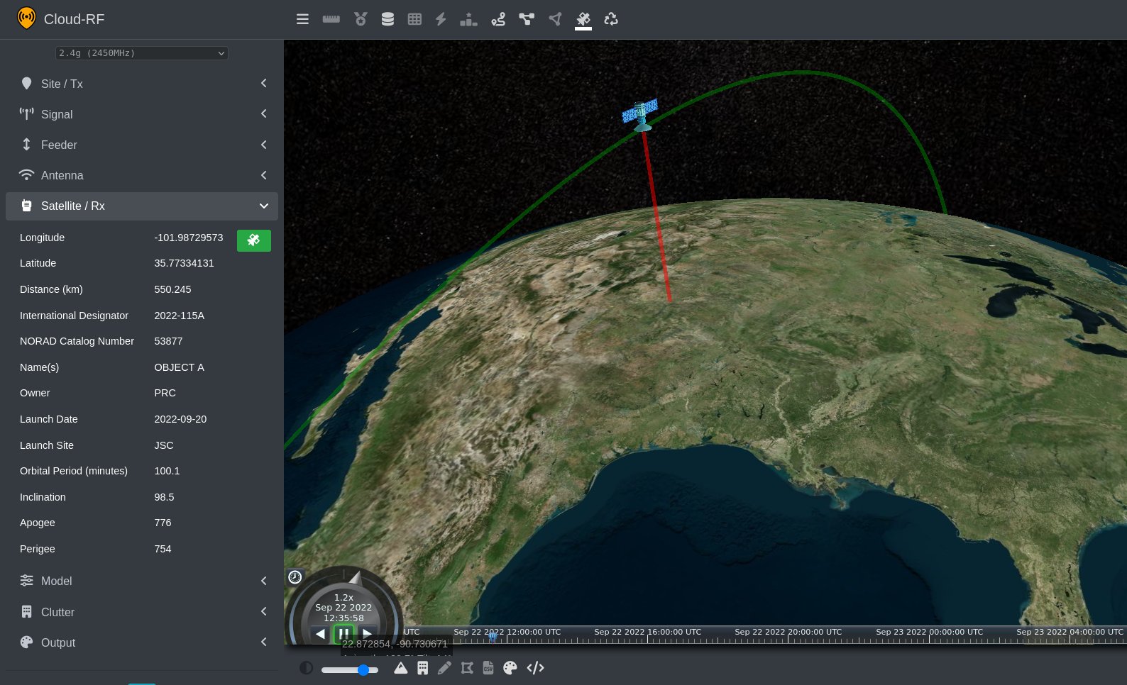
400km radiusCustom WMSJSON templatesCustom WMTSSatellite data
With 19 new features/improvements and 69 bugfixes in this period, the user interface has matured considerably due in large part to user feedback from the community. We’ve said no to a few feature requests also which is necessary to keep the interface technology agnostic and easy to use. That doesn’t mean we can’t support complexity or special waveforms directly in the API.
Radius increased to 400km for aircraft (3.0)
GPU engine integrated with best server and CSV analysis tools (3.0)
New 300m resolution for airborne broadcasting (3.0)
Received Signal Received Power (RSRP) option added to measured units (3.1)
Account information dialog (3.2)
GPU Best Site Analysis (3.2)
Custom WMS and WMTS map sources (3.4)
Satellite database updated (3.4.2)
Multi azimuth antenna patterns (3.5)
Route, multipoint and path path tools updated for all possible measurement units (3.5.1)
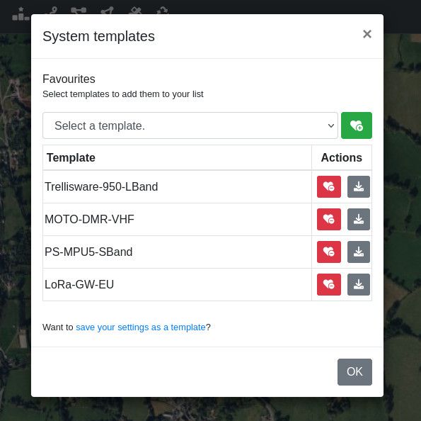
JSON templates system (3.6)
The long surviving Google Earth interface lives on and has been given a fresh wind thanks to code compatibility libraries which mean we no longer have to worry about breaking it with new Javascript. Long live Google Earth!
UI Changelog
## Version 3.6.1 (2022-11-28)
- Fix: Layer from archive would not load when clicking on the layer name or selecting "Add tower(s) only to map" button.
- Fix: Processing modal window getting stuck when using the Interference or Super Layer tools.
- Fix: Display the power of items loaded from the archive in the selcted power unit.
- Fix: Dynamically move navigator controls down to make space for imagery layer list.
- Fix: Prevent crash when disabling path profile analysis before calculation completes.
- Fix: Refreshes displayed clutter after deleting all clutter using the clutter manager.
- Fix: Selecting a template in the Google Earth interface crashes.
- Fix: MANET nodes sometimes clipped by the terrain resulting in partially hidden markers.
- Fix: Best site analysis tool sometimes goes into "zombie" state under bad network conditions.
## Version 3.6 (2022-11-10)
- Feature: Templates functionality makes use of the new API endpoints and JSON files.
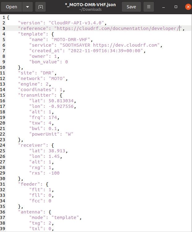
- Feature: Added button to download the JSON template for both custom and system templates.
- Feature: Added modal to add/remove favourite system templates.
- Feature: Dropdown select of templates indicates if the template is a system or custom template by prepending with either "System" or "Custom" respectively.
- Fix: Styling issues on custom template save/delete modal.
- Fix: Reorganised "My Account" modal as was becoming cluttered. Logout button moved to top and managers split into a single row. API usage moved to the bottom.
- Fix: Some API errors which are returned as an array of values would not be parsed as an array, instead the error displayed would be a generic "Request failed." message which wasn't indicative of the error.
- Fix: Don't fire a GPU request when loading a GPU template.
- Fix: Adjusting the `rxs` field manually would not update the receiver sensitivity slider.
## Version 3.5.1 (2022-10-31)
- Feature: Route, Multipoint and Path tools able to display SNR, dBuV and RSRP units as well as dBm.
## Version 3.5.0 (2022-10-18)
- Feature: Multi-azimuth antenna support by sending a comma-separated list of values, for example, `0,120,240`.
## Version 3.4.2 (2022-09-21)
- Update: Satellite database updated to 2022-09-22.
- Feature: Fly to PPA when loading from the archive.
- Fix: Custom pattern vertical beamwidth not visible in the Google Earth interface.
- Fix: Profile drop down not populated and opening the clutter manager in the Google Earth interface.
- Fix: Sensitivity is loaded when selecting a template.
- Fix: Map attribution interfered with satellite timeline controls.
- Fix: Loading PPA from archive and then hovering over chart would cause a crash.
## Version 3.4.1 (2022-09-14)
- Fix: Template saves coax type.
- Fix: Problem toggling the azimuth mode in the Google Earth interface.
- Fix: Problem loading a template in the Google Earth interface.
- Fix: Switching between templates with engine set to GPU and CPU runs area calculation with incorrect engine.
- Fix: Saving a custom map URL cuts off part of URL after an "&".
- Fix: Suspends error logging when library blocked by client.
- Fix: Handle missing preferences.
## Version 3.4.0 (2022-08-31)
- Feature: Custom WMS and WMTS URLs for imagery layers.
- Feature: Attribution text lists API providers.
- Fix: Pruned dead and unsuitable map sources, such as "Blue Marble".
- Fix: Problems with editing coordinates.
- Fix: Antenna patterns not loading properly in some browsers.
## Version 3.3.0 (2022-08-23)
- Feature: Sets free space model with diffraction off and shows warning for best site analysis.
- Feature: Select last network when opening archive to match the last row.
- Feature: Make clutter go to ground.
- Fix: Improved area calculation error handling.
- Fix: Selecting a network in archive drop down when some items have no network would cause a crash.
- Fix: Legacy colour key images not displayed.
- Fix: Super layer KMZ quick-download button fixed for "Merge network"
## Version 3.2.0 (2022-08-15)
- Feature: Account Information dialog.
- Feature: GPU Best Site Analysis.
- Fix: Updates to colour schemas to match recent changes to colour schema API.
- Fix: Buildings layer cannot be removed.
- Fix: Receiver sensitivity icons missing.
- Fix: Creating a clutter profile does not refresh the list.
- Fix: RSRP breaks MANET.
- Fix: Opacity slider doesn't work.
- Fix: MANET reload by name click and best server for imperial units mi/f.
- Fix: Crash clicking layer checkbox while layer is loading.
- Fix: Default RSRP schema not always selected.
- Fix: Interference tool is trying to map colours to colour key.
- Fix: Crash saving clutter polylines with less than 2 coordinates or polygons with less than 3 coordinates imported from kml.
- Fix: Crash downloading MANET metrics report when node evauation failed.
- Fix: Power unit in MANET node details dialog displayed as undefined.
- Fix: Node percentanges on MANET metrics report sometimes NAN.
- Fix: Points CSV validation no longer works.
- Fix: Entity already exist in collection when disabling MANET.
- Fix: Crash adjusting bsa sliders when result loading failed.
- Fix: BSA images not recoloured on colour schema changed.
- Fix: Custom antenna polar plot not displayed in Google Earth.
## Version 3.1.0 (2022-07-18)
- Feature: Added Received Signal Received Power (RSRP) as an option to the "Measured Units" dropdown.
- Fix: Deleting multiple selected networks will now give the name of the networks rather than the ID.
- Fix: Selecting a PSK/QAM modulation will only show supported PSK/QAM bit-error-rate values, and likewise when selecting a LoRa modulation.
- Fix: Deleting a network from the archive now gives a better modal message rather than a browser `alert()` window.
- Fix: Occasional crash when computing azimuth and tilt for the mouse tootltip for satellite mode when the position has not been computed yet.
- Fix: Can't find variable `Map` in Google Earth interface.
- Fix: Crash in Google Earth when logging error information.
- Fix: Prevents crash in Google Earth interface when changing clutter profiles.
- Fix: Formatting issue in Google Earth.
- Fix: Helper dialog describing channel noise adjustment when changing bandwidth
- Fix: Tx Height AGL and RF Power textboxes extending over unit drop downs.
- Fix: Crash in Google Earth interface when you change properties that would update the map location when in web UI.
## Version 3.0.1 (2022-07-06)
- Feature: Added support for 180m and 300m resolutions.
- Fix: GPU is populated in dropdown of processing engines when GPU isn't available.
## Version 3.0 (2022-07-04)
- Feature: Radius limit now 400km.
- Feature: GPU processing no longer handled through WebSocket, instead goes through the same API as CPU processing for simplicity. Removed button to close GPU processing engine, instead you now just switch back over to CPU mode from the dropdown in the "Output" menu.
- Feature: Integration of GPU engine with other tools including best server and CSV import.
- Fix: Colour schema list gets populated with some empty values when using GPU mode.
- Fix: Prevents failure on area calculation due to invalid input from logging an error.
- Fix: Interference dialog not always populating networks.
- Fix: Duplicate entry for gpu in the engine drop down.
- Fix: Some antenna patterns were not being saved in templates.
API changes, v3.0 June to 3.6 November
With 30 improvements and features and 28 bugfixes, the API has largely remained the same from a developer’s perspective but it now has more consistency between the CPU and GPU engines, more choice with defining antenna azimuths and more useful error messages to help developer’s make better choices and save time.
Under the hood, the ATAK interface has had a major refactor to support customer’s official TAK Server’s with our infamous chatbot. A new chatbot management interface has been especially created which can validate certificate chains using OpenSSL to warn of issue before you get to them eg. “This certificate is invalid” or “This key is incorrect” or “Cannot ping your TAK server”.
Offline JSON file templatesMulti-Azimuth requestsBest Site Analysis for ATAK
GPU integration
The new GPU engine has received several updates throughout this period to add models, gains, antenna patterns, multi-azimuth patterns and output styling inline with the CPU engine, SLEIPNIR.
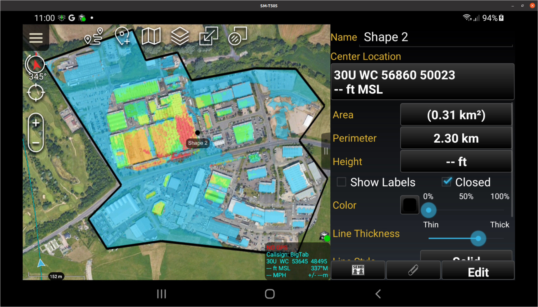
In September, the powerful Best Site Analysis capability was integrated with ATAK. When the SOOTHSAYER bot is connected to the TAK server, any polygon sent to it will generate a BSA layer.
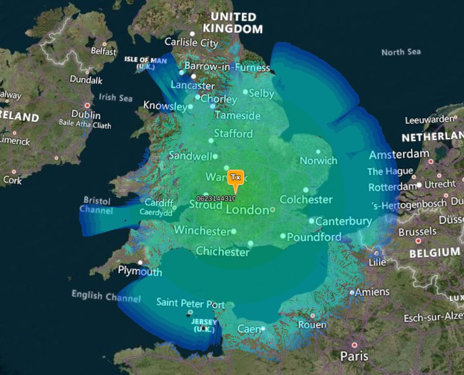
Due to demand, the maximum radius for the GPU engine was increased to 150km to support broadcasting. During GPU testing we were generating 100 mega pixel (100,000,000 points) heatmaps in a few seconds which is too large for a client. We are working on a scalable solution to visualise images of this resolution as an image pyramid.
SLEIPNIR mods
The SLEIPNIR CPU engine is now at version 1.6.1 and has conditional smoothing of coarse DTM, knife edge diffraction from clutter (note we already do this for surface models) and slightly (3dB) more optimistic diffraction following feedback from a mountain rescue team.
Received Signal Received Power (RSRP) is not native to the engine instead of the API and the reliability variable can now be used for non-ITM models to provide a 10dB tuning margin where 50% is 0dB and 99% is 9.9dB path loss.
The maximum radius has been increased to 400km for airborne platforms. To support the larger radius, we’re also offering a new low resolution of 300m.
API management
The V1 “URL” API will be retired at the end of this year. Users who have integrated with this API should migrate to the new JSON API as soon as possible. The new JSON API has been powering the web interface for almost two years.
## Version 3.6.0 (2022-11-25)

- Deprecation: Added deprecation message to `v1` API endpoints. The `area` and `path` will be removed on the 31st December 2022. Please migrate any scripts to the new JSON API and see https://cloudrf.com/documentation/developer/
- Fix: Chatbot welcome-storm with other chatbots.
- Fix: Obsolete paths on terrain coverage map and HTML PPA response.
- Fix: Improvements to automation testing.
- Fix: Sending malformed JSON to a `v2` API endpoint now returns a useful error message.
- Fix: Deprecated `v1` API endpoints were incorrectly counting API credits.
- Fix: Power value of 1mW for GPU fails.

## Version 3.5.0 (2022-11-10)

- Feature: Moved from database-driven to JSON-driven templates with new API endpoints to manage custom templates.
- Feature: System templates can be retrieved and saved as a favourite using new endpoints.
- Fix: Race condition on GPU processing files as its so damned fast.
- Fix: Public shares for GPU layers needed reprojecting to EPSG 3857.

## Version 3.4.0 (2022-10-18)

- Feature: Gain support for GPU engine.
- Feature: Antenna support with azimuth and tilt for GPU engine.
- Feature: Multi-azimuth support for antennas by sending a comma-separated list of values in the `antenna.azi` value, for example, `0,120,240`.
- Fix: Path tool on TAK successfully returning only about 50% of the time.
- Fix: Area requests to `v1` API returning colour key data in improperly formed string values.
- Fix: `clutter` command on TAK chatbot working again.
- Fix: Resolved issue with custom colour schemas and low resolution screens.
- Fix: Sanity check ADF files.
- Mod: Default clutter templates adjusted. Urban height reduced to no more than 2m.
- Mod: GPU engine max radius capped at 10km (CPU max = 400km).

## Version 3.3.0 (2022-09-22)

- Feature: Support for TAK server 4.7 through Chatbot and ATAK.
- Feature: Extended response information when executing `id` to Chatbot through ATAK.
- Feature: Support for GPU BSA on Chatbot with the multipoint tool through ATAK.
- Feature: Added new chatbot manager to spin up chatbots on demand which interact between TAK servers and API.
- Feature: Extended preferences functionality to allow for custom imagery.
- Feature: Delete all clutter button added to clutter form.
- Fix: Processing engine saved in templates.
- Fix: Commercial restrictions messages now return HTTP 403 (Forbidden) rather than HTTP 400 (Bad Request).

## Version 3.2.0 (2022-08-15)

- Feature: System colour schemas no longer able to be deleted by a user so that users will always have a list of schemas to choose from.
- Feature: Height ceiling increased to 120km over 60km.
- Feature: When using Greyscale GIS colour schema no longer returns validation error for mixing outputs and schema.
- Feature: Improvements to the PPA KMZ export with fresnel support and new icons for transmitter, receiver and obstructions.
- Fix: Improvements to the functionality of the colour schema generator.
- Fix: Creating a BER colour schema fails with a HTTP 500.
- Fix: Update to `preferences` stripping out underscores from colour schemas.
- Fix: Google Earth layer no longer allows to manage colour schemas. Added notice with workaround instructions.

## Version 3.1.0 (2022-07-18)

- Feature: Improvements to `preferences` to extend to additional values and give information about a users plan.
- Feature: Improvements to precendence of preferences, where in some cases a previous request values will be taken over a users preferences.
- Feature: Colour palette bucket limit increased to 75.
- Feature: Return request to `preferences` as a correct JSON response.
- Feature: Users with a private server will now be indicated when they make a request to `preferences`.
- Feature: Colour pallette creator extended to support Bit-Error-Rate measured units.
- Feature: Bit-Error-Rate modulation extended from 10e-6 to 10e-8.
- Feature: Allowed support for Received Signal Received Power (RSRP) measured units with an `out` value of `6`.
- Feature: Added default RSRP colour key.
- Feature: SLEIPNIR 1.6.1 calculates and returns (LTE) RSRP if selected
- Feature: SLEIPNIR 1.6.1 uses reliability for non-ITM models with a 10dB range. 50% = +0dB, 99% = +9.9dB
- Fix: Successful deletion of networks in the archive are returned with a success `message` rather than `error`.
- Fix: Correct names of plans when making a request to `preferences`.
- Fix: BER colour palette in JSON response was missing unit.
- Fix: Improvements to the default `PATHLOSS.dB` colour key.
- Fix: Hata model high-plateau issue resolved in SLEIPNIR 1.6.1

## Version 3.0.1 (2022-07-06)

- Feature: Resolution supported up to 300m.

## Version 3.0 (2022-07-04)

- Feature: Improvements to GPU processing with the use of remote processing nodes.
- Feature: GPU produced images are now styled in the API based on the specified colour schema.
- Feature: Extended `data` API to retrieve a tile based only on tile name.
- Fix: Logic issue with users mixing credits and plan was incorrectly refusing service to users with expired plans, but spare credits.
- Fix: Custom clutter profiles are created with the list of 101 to 199 clutter codes.
- Fix: Obtaining height data from OpenStreetMaps would sometimes fail.
- Fix: KMZ download failing on equator
As communications systems have grown in capacity, they have expanded in physical bandwidth in an increasingly congested RF spectrum.
Effective digital communications planning requires more than knowledge of antennas and propagation fundamentals. It now needs an intimate understanding of bandwidth and noise to co-exist and communicate efficiently.
Unfortunately, this key aspect of modern RF systems is often taught badly, or in some cases not at all, leading to often unwelcome surprises for equipment operators in the field. As a technology and market agnostic platform we’ve observed poor bandwidth knowledge in many markets, but notably MANET and 5G, both of which are accelerating the deployment of wideband systems, often with little to no planning beyond a topographic map study.
Both radio markets are evolving from narrower channel technologies, which in the case of MANET and the VHF Combat-Net-Radio (CNR) it replaces was measured in KHz so they need to update their theory training content and associated software to convey these potentially complex topics to novice students in a digestible manner.
Increasing bandwidth increases noise, which reduces coverage
Teaching noise
As bandwidth increases, so does channel noise. This simple concept might seem easy to remember for a student but without visual aides, and since the demise of analog systems; audible aides, it is hard to demonstrate in practice.
A good teacher may show visual aides like noise charts, FFTs, spectograms and a bad one may show some Johnson-Nyquist formulas buried within an all-day powerpoint which is not helpful except for getting paid.
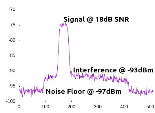
FFT showing a narrow signal and wideband interference
A student can tick the right box on their exam(s) but spend their career wasting bandwidth and struggling to establish communications because they believe that big is better – it isn’t, or worse still, that bandwidth has no effect on the coverage since that’s a function of transmitted power and/or height. Having an intimate understanding of the interplay between bandwidth, receiver sensitivity and thermal noise will make spectrum users more efficient, effective and considerate.
Bandwidth MHz
Thermal noise (dBm)
0.1
-124
1
-114
2
-111
4
-108
8
-105
16
-102
32
-99
64
-96
Bandwidth thermal noise table based on a temperature of 21C
Which waveform is best?
Comparing digital radios is complicated due to the myriad of features, waveforms and software.
Given a particular waveform it will have characteristics such as a minimum Signal-to-Noise Ratio (SNR) value which it requires to achieve a symbol rate necessary to deliver a fast data link for example. This dB value must sit proud of the noise floor so if the noise floor is high at -90dBm, coverage will be reduced and conversely, by taking it to somewhere quiet eg. -110dBm, the coverage will improve by 20 decibels – a huge difference.
To compare waveforms precisely, the same noise floor should be simulated, initially, with fixed values to eliminate random error in field testing. The sensitivity values will be somewhere between 3 and 20dB depending on what the waveform and target Bit-Error-Rate (BER) is.
Bit Error Rate (BER) describes the ratio of errors in a data stream. An ok value is 10-3 or 1 bad bit in a 1000 or 0.1%. This increases with noise until a signal is unrecoverable. For more on BER see an older blog here.
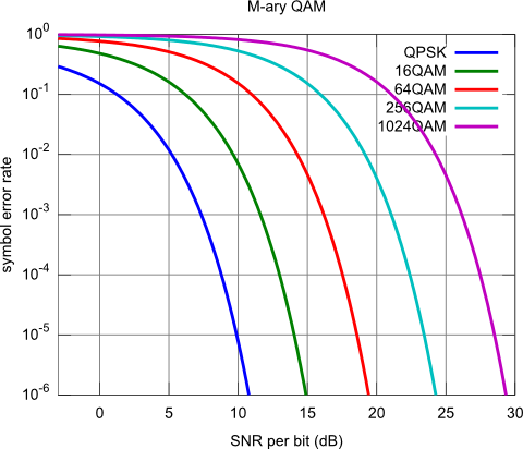
For ground radios designed for noisy environments, a BER of 10-2 (1 error in 100 or 1%) is used here for extracting our planning thresholds from a chart of SNR curves. For an airborne system without obstacles this could be higher, for example 10-5.
Signal to Noise Ratio for different modulation schemas against error rates.
A narrow waveform eg. QPSK gives better coverage and works better in noisy conditions. This is the fallback telemetry mode used in many data radios.
A wide waveform eg. QAM64 is capable of better throughput and delivering high bandwidth streams such as HD video.
The best radio is one which can use different waveforms to satisfy both coverage and capacity.
Modelling bandwidth: A tutorial
Modelling RF Bandwidth and noise
Quick reference guide
A quick reference guide for using bandwidth and noise is available here. For other guides see here.
Bandwidth and noise is essential knowledge for anyone deploying wideband systems or comparing waveforms.
RF theory training can be enhanced (and needs to be) with visual tooling to let students quickly observe the impact of different inputs in a controlled environment with templates to minimise user error.
For information on how SOOTHSAYER can help with signals training see here.
Smart farming is using Internet of Things (IoT) technologies in agriculture to enable efficient use of resources.
For this blog we’re focused on cattle farming on large, fence-less farms in New Zealand. The farms in question are vast and remote so connectivity options are limited. This is why an off-grid sub-GHz LPWAN network is ideal due to its long range and the requirement to only send small, infrequent, packets of data.
For the solution to be cost-effective compared with Satellite, as little infrastructure as possible is needed which in this case is a LPWAN gateway on a pole, some collars for the herd and an app to manage the system via a web service.
Siting the LPWAN gateway(s) properly is critical to achieving not only coverage across the farm(s) but to reduce the number of gateways, which reduces complexity and cost.
Sub GHz LPWAN on the farm
An 868MHz LPWAN signal can go for many miles under the right conditions. We know this well from powering the Helium LPWAN network’s planning tool, Helium Vision, where people can communicate data 50 miles with a fraction of a watt of RF power and an omni directional antenna.
Despite it’s useful diffraction properties which enables it to work non-line-of-sight (NLOS), it’s still sensitive to obstructions so clutter on the farm such as buildings and trees needs modelling accurately. CloudRF has 10m Landcover for New Zealand from the European Space Agency and 10m DSM from the LINZ Geospatial agency.
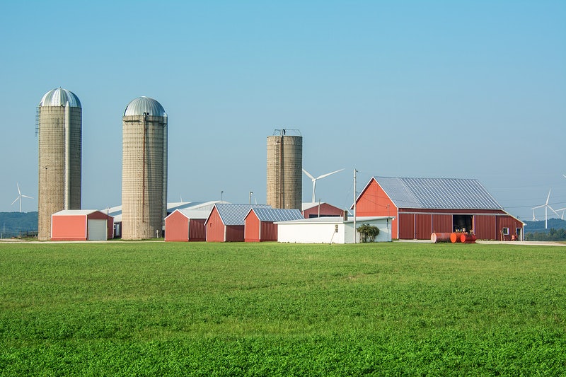
These data sets are adequate for most outdoor scenarios but are not fine enough to model a farm complex of buildings, such as tall grain silos, metal sheds and seasonal obstacles. For high resolution you could source your own surface model, as our customer Halter did…
Farm buildings and silos
Use case: Halter
Halter are a novel agri-tech startup focused on cattle management with a unique solar powered collar.
They needed accessible RF planning software to help their engineers site LPWAN gateways. Having used and liked Cloud-RF, they needed higher resolution surface models of the farms, and no pesky API restrictions!
They also planned to build their own tools on top of our powerful physics based API which is smart as it allows their R&D team to focus on their primary product, and not waste time reinventing the wheel.
Their options were either buy expensive commercial data or self generate data using a drone and photogrammetry software such as Pix4D. Given the prohibitive cost of high resolution commercial LiDAR, it would only take a few jobs to make a return on the purchase of a decent drone!
Halter purchased a private Keyhole Radio server from us which included the API they needed. The server runs as virtual machine and crucially, lets them import their own terrain data.
They were quickly able to import high resolution, organic data into their server as GeoTIFF files. This allowed them to work with data which was very current, even hours old, so would be an accurate model of tree heights and man made obstructions.
The terrain format accepted by Keyhole Radio and SOOTHSAYER is GeoTIFF, Int16 resolution and WGS84 (EPSG:4326) projection.
LPWAN coverage on a farm in New Zealand
1m resolution
It wasn’t all plain sailing though, they found that there was a limit to the physical tile sizes our server could use caused by memory. The solution was to reprocess the large tile into smaller tiles to make it digestible.
A 5000 x 5000 GeoTIFF at Int16 resolution will require 50MB of disk space. If this is 5m LiDAR, the physical width is 25km x 25km. Our engine can super-sample, so if you used this tile, but requested 1m resolution, it would create a raster in memory measuring 25,000 x 25,000 pixels which would need 1.25GB of memory.
For 1m resolution however, tiles measuring 1000 x 1000px would only require 2MB of disk and memory. You may need to load in a few, lets say 16, to do your model but that’s still only 32MB.
You could also resolve this by increasing the memory available to the server but it’s recommended to prepare data into smaller parcels. We support 1m resolution in our API but don’t hold a lot of 1m data sets due to their substantial cost and size. If you already have 1m data, a Keyhole Radio or SOOTHSAYER server is the answer.
1m resolution
Summary
Cloud-RF’s powerful API is ideal for efficient smart farming.
Our private servers will let you take it to the next level with terrain data you can source yourself, no API restrictions and as a bonus, they work without an internet connection!
We took a field trip to model LTE (4G) coverage in order to collect data we can use to develop calibration utilities and improve modelling as modelling is only as accurate as your inputs.
We focused on a single remote cell in the Peak District national park identified through cellmapper.net. We expected to find one cell only but were surprised to be serviced by several distant LTE cells, not evident in the crowd sourced app and equally significant, we established limited or no coverage in an area where a national map suggested coverage was available.
Key findings
Data revealed the crowd-sourced coverage app was conservative in rural areas
Data revealed the operator’snetwork map was optimistic in rural areas
Modelling was matched with 2.5dB RMSE for a cell 12km away
Modelling was on average accurate to 5.5 dB RMSE
Improvements to modelling have been identified
Equipment and process
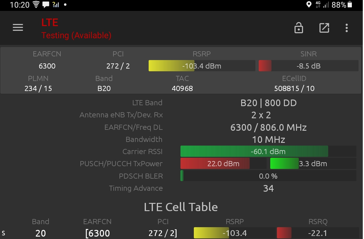
We used a rooted Samsung Galaxy Tab with an integrated Qualcomm X11 LTE modem, running both Network Signal Guru (NSG) and Cellmapper. NSG requires root access to lock to a cell which was necessary to prevent our survey tablet from hopping around not only protocols (2G,3G) but neighbouring cells.
Cellmapper is a crowd-sourcing app which writes signal strength readings to a CSV file, convenient for our analysis. Before embarking we planned a route around a remote cell on the edge of available coverage maps.
Both apps record various LTE power levels such as Received Power Received Signal (RSRP), Received Power Received Quality (RSRQ) and Received Signal Strength Indicator (RSSI). For this test we use RSSI which is typically a stronger value than the others as it is the measured carrier, irrespective of bandwidth.
Cellmapper
Network Signal Guru
Receiver measurement calibration
Radio receivers are subject to measurement error, typically in the range of 0.5 to 3.0dB for very expensive and consumer grade equipment respectively. As we were using a consumer grade Snapdragon 662 SoC with an X11 LTE modem, we needed to find out it’s measurement error. The Qualcomm datasheets we could find didn’t list this value so we used empirical measurements to establish it.
During our survey we paused at a site 3km from a tower with line of sight where we recorded continuous power readings with the tablet static on the ground for about 15 minutes. Consistency is essential for calibration. We have analysed these readings to establish a standard deviation in readings of 3.1dB for the X11 LTE modem, which puts it at the consumer end of the spectrum for survey device accuracy, in accordance with its price.
We use the error of 3.1dB in our analysis by subtracting it from the Root Mean Square Error (RMSE).
Setting off uphill from Derwent Dam car park with Sheffield’s man-of-the-mountain, Chris, we approached our target cell located on the hillside below us.
As we neared 500m we used NSG to lock onto a strong LTE signal which we believed was the target (CID 130256660, PCI 270), based on proximity and strength (-60dBm RSSI). It was in fact a tower on a distant hill 12 km to the south with line of sight, CID 131413770. Surprise number 1.
Field testing in the Peak District
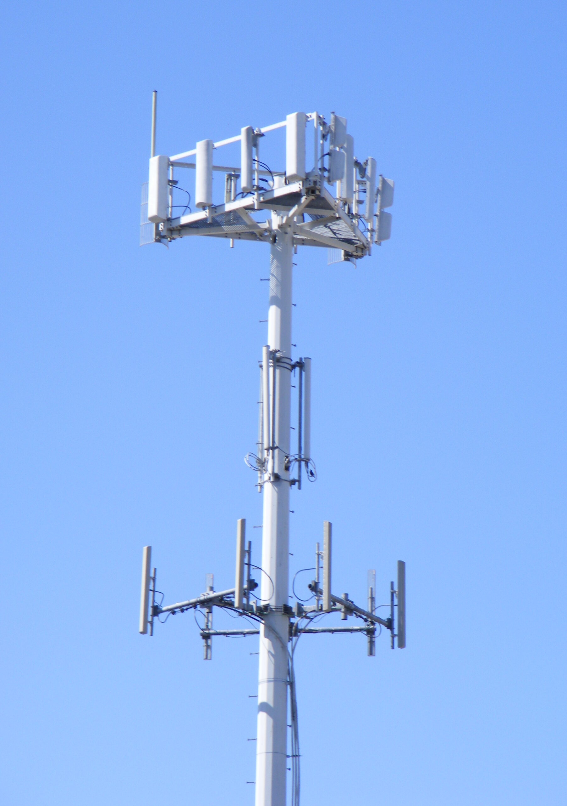
At the top of the hill we could see the target tower’s directional panels which confirmed it was configured to serve the A57 “Snake pass” road below. One panel was oriented north-west towards Manchester (CID 130256660) and the other south-east towards Sheffield (CID 130256650). Based on the dimensions of the panels we estimated their beamwidth as at least 120 degrees and gain of at least 10dBi.
As we passed the eNodeB along the hill top we were conscious of a number of cell neighbours and performed a targeted re-selection where we ended up briefly attached via the antennas back-scatter of *6650, made possible by our proximity. This didn’t last for long before we re-selected to a strong signal (PCI 337) which we were convinced was CID *6660. It wasn’t. Surprise number 2.
Surveying LTE cells with Network Signal Guru
We later found out this was also a distant cell with line of sight near Hope, 7km due south of us!
Marching on happily with a great signal, we started a gentle descent until we lost the horizon behind us. At this point the neighbours we observed disappeared and our serving cell (in Hope) became very weak as we entered the signal’s (diffracted) beyond-line-of-sight (BLOS) shadow. As predicted in the video based on the surrounding high plateau we could see, we lost the signal as we continued to head north toward Alport Castles, a local feature. We descended into the valley below without a signal (despite a national map suggesting otherwise) and continued the next 3.5km without any coverage at all 🙁
Losing all cells on a high plateau
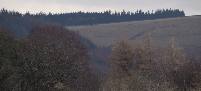
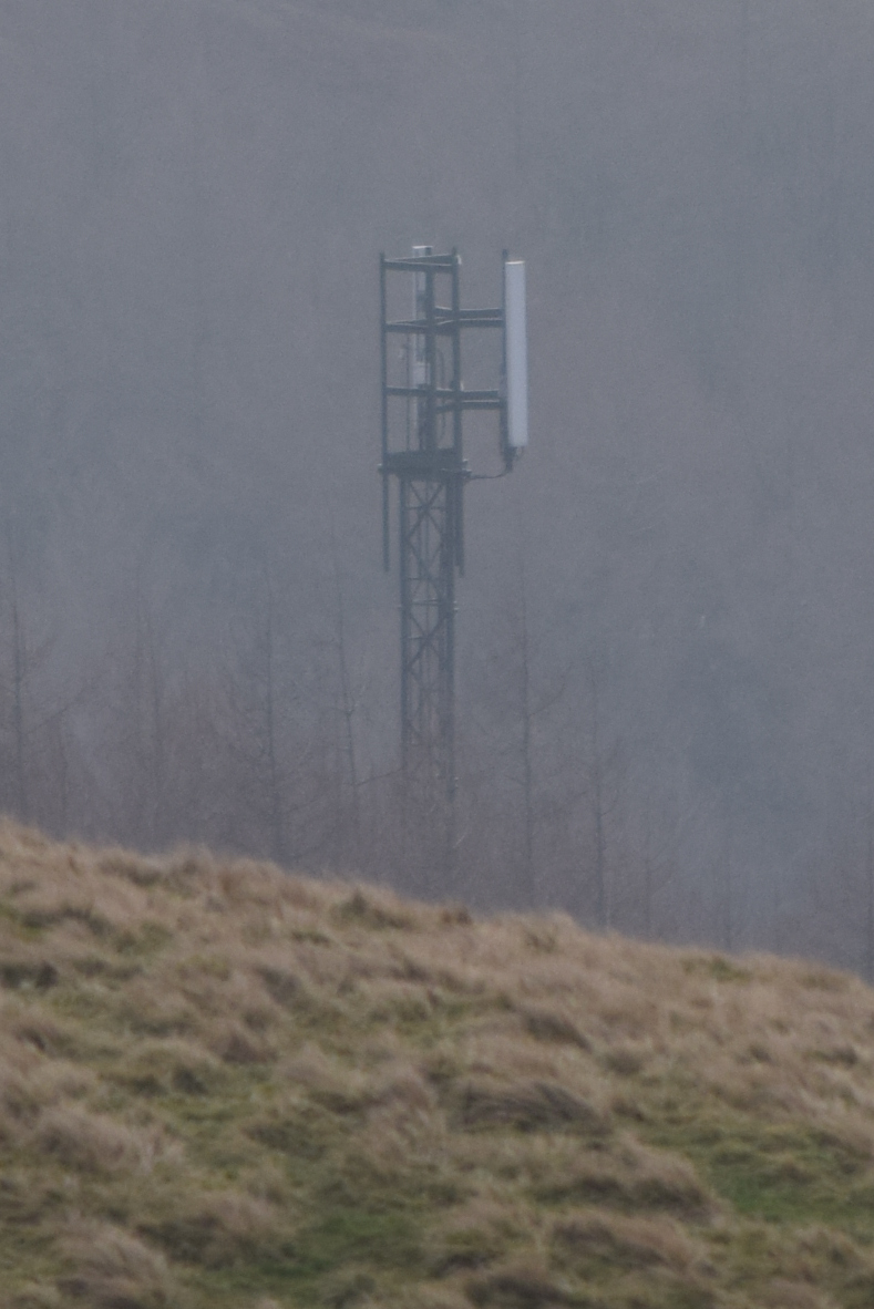
As we exited the remote valley, heading towards the A57 road, we reacquired a signal and finally locked onto our target, *6660, with an excellent signal and line of sight (Credit to Chris for spotting the tower in the trees at 2.7km!). As observed, the directional pattern was focused on the road and we were in the main beam.
The elusive target cell!
Acquisition of the target cell
A quick map study and we elected to march west until we lost the signal. This event occurred after only 1.5km thankfully as we hand railed the road over undulating terrain. We followed the same route back to the acquisition point which doubled our measurements for this section.
Confirming the direction of the powerful 10MHz LTE800 bearer with a portable spectrum analyzer with a bad LCD.
From the A57, in the main lobe, we climbed the hill to the south east and headed back toward the target cell. Knowing it had a directional pattern, we anticipated signal strength decreasing as we exited the main lobe which we confirmed as we drew parallel with the cell, eventually circumnavigating it to the south.
As we exited the beam of *6660 and entered the influence *6650 we re-selected for the final phase of our journey which would take us into a steep ravine and then up the hill, right past the cell.
A sweaty climb up a steep hill behind the cell, saw signal strength and field testing enthusiasm collapse which was fixed with some fizzy snakes. We lost the cell for good only 500m behind it due to the convex hill and directional pattern.
Moral of the story is, in RF, proximity to an access point is no guarantee of service!
Serving cells
Hagg Farm eNodeB
Cell ID
PCI
Location
Technology
Frequency
Comments
130256650
272
Hagg Farm (South East)
LTE Band 20 10MHz
806MHz DL
~15m AGL
130256660
270
Hagg Farm (North west)
LTE Band 20 10MHz
806MHz DL
~15m AGL
131377930
337
Hope Quarry
LTE Band 20 10MHz
806MHz DL
~15m AGL
131413770
441
Little Hucklow
LTE Band 20 10MHz
806MHz DL
~20m AGL
Table of serving cells featured in our data
The cells all have a downlink and an uplink frequency. As these four cells share the same downlink they are separated in time using a multiplexing schema and the Physical Cell Identifier (PCI) code. If we only took out a spectrum analyser we’d never know which cell we are looking at otherwise.
Data analysis
We chose to model after field testing. We could have done it before but it would have ruined all the surprises that came up during analysis like the serving cell 13km away!
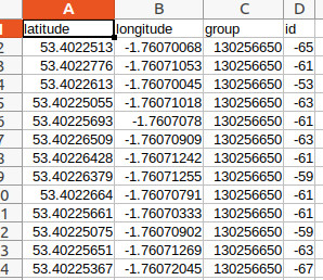
We extracted the CSV data (1034 rows) from the survey tablet which for cell mapper was located at /storage/emulated/0/Android/data/cellmapper.net.cellmapper/files/.
We sorted it by cell and created clean CSV files for each cell with only the location and RSSI.
Cellmapper CSV survey data
Gap analysis
Formatted CSV data. group = CID, id = RSSI
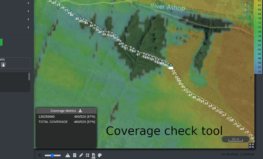
We used our new “coverage check” CSV import tool. This tool allow the import of customer locations which can be tested against visible coverage layers to report a correlation.
This is a binary yes/no comparison with a summary report eg. “87% coverage” which is handy for comparing options.
It cannot automatically calibrate field test measurements but is useful for gap analysis as a “first pass” toward calibration.
This tool is handy for manually aligning the modelling until it matches visually but is too simplistic for calibration.
Coverage check tool showing an 87% correlation. The deadspot is where modelling was conservative.
Fine tuning inputs
Our confidence level for the inputs started around 50%, based on known frequencies, heights and power levels for the UK network. For the first cell, we used a combination of known, observed and assumed values.
You can be forgiven for thinking why not do field testing with known transmission parameters but even then you must calibrate as old batteries, weathered connectors and battered antennas will all impact a transmitters actual effective radiated power (ERP).
As we working LTE800 we used the ITM model, designed for this UHF band when it was conceived for TV broadcasting. This general purpose model has built in diffraction and also has a reliability variable which we can use for fine tuning.
Known values: frequency, location, approximate height, approximate azimuth Estimated values: Antenna azimuth, beamwidth, gain, RF power, exact height
Once we had a coverage plot using some sensible power values and the coverage-check tool reported a correlation > 90% we rendered it using the Greyscale GIS colour schema and download a GeoTIFF raster. This contains fine grain signal values to 1 dB resolution.
Calibration process
We suggest this workflow for the calibration process.
We also have an API capable of returning data in open vector and raster formats including SHP and GeoTIFF so there are other ways to do this...
Gap analysis with the coverage check tool in the web interface and approximate/rough inputs
Power balancing with the path profile tool for selected points only (Recommend a LOS link at long range)
Gap analysis with the coverage check tool in the web interface and power balanced inputs
Regenerate the layer with the GIS schema and export for precision offline calibration
Make minor (1-2dB) adjustments to either the loss or gain values for LOS links, and/or clutter profiles for BLOS until the calibration script reports an RMSE value < 10.
Offline calibration
Using a Python script and the rasterio library we were able to query each row from the CSV data against the GeoTIFF raster instantly, negating the need for many recursive API calls.
The offline method is more efficient when working with large point-to-multipoint layers and spreadsheets than calling the API directly. It computes a mean error which can be positive or negative and a more useful root mean square error (RMSE) which is always positive. A lower figure is better with 0dB being ideal (and also impossible).
The API method is still valid for testing select points or calibrating dynamically.
python3 Offline_Calibration.py 131413770.csv 131413770.tiff
...
Lat: 53.402250 Lon -1.760703 Measured: -65.0dBm Modelled: -68.0dBm Error: 3.0dB Mean error: 0.5dB
Lat: 53.402252 Lon -1.760699 Measured: -59.0dBm Modelled: -68.0dBm Error: 9.0dB Mean error: 0.6dB
Lat: 53.402253 Lon -1.760699 Measured: -61.0dBm Modelled: -68.0dBm Error: 7.0dB Mean error: 0.7dB
Lat: 53.402252 Lon -1.760698 Measured: -63.0dBm Modelled: -68.0dBm Error: 5.0dB Mean error: 0.8dB

Model error is mean 0.8dB, pure RMSE 5.6dB based upon 84 measurements
Receiver measurement error: 3.1dB
RMSE adjusted for receiver error: 2.5dB
The modelling inputs are excellent.
RMSE
Description
Comment
0 to 3
Excellent
Calibrated!
3 to 6
Very good
Inputs are very close. Fine tuning needed.
6 to 9
Good
Inputs are good but more tuning needed
9 to 12
OK
Inputs are OK but not tuned
> 12
Bad
Inputs are bad. Check basics eg. Height, Frequency, Power
Suggested interpretation of calibration scores. Requirements will vary by scenario.
The results
We achieved results better than expected. We were aiming for under 6dB RMSE and achieved 3dB, at 7km range, which is excellent, and coincidentally as accurate as the measurement accuracy of our survey device.
Manual calibration can be time consuming, and collecting good data definitely is. We felt we could have improved the scores further with more data, like the antenna data sheets for starters, but were happy with our 3dB.
The good
The best results came from the distant cells where LOS was achieved. This makes sense as without obstacles to complicate things the path loss decays at a predictable rate, based on wavelength, which can be plotted as a clean curve. Once we had this power balanced using the path profile tool and manual adjustments, it produced a great match with the data due to the open nature of the high plateau.
Calibrated modelling for a cell 7km away with line of sight
The ugly
The other cells, like our target at Hagg Farm (South east), served a more complex piece of ground in the valley which had steep ravines and tall trees. As expected we didn’t fair as well here and achieved 10dB RMSE. Analysis of where we lost accuracy can be summarised as follows:
Trees. We found 2m LiDAR to be too conservative here as this contains the tree canopy. We tried smoother DSM with clutter profiles which gave a better result but didn’t go as far as adjusting our clutter profile. This is a future trees blog!
Proximity. Counter-intuitively, being closer to the cell is not better for measurements and calibration than being further away. This is due both to the way path loss decays on a curve and the highly directional panels cells use. Small differences near a cell produce large differences in data, compared with very small differences up on the plateau with the distant LOS cells. We can model directional panels but are guessing what the *actual* beamwidths are.
Cell
Points
Mean
RMSE
130256650
164
-0.7
9.8
130256660
460
0.9
6.9
131377930
127
-1.6
3.0
131413770
84
0.8
2.5
TOTAL
835
-0.15
5.5
Table of scores for the calibration of the four measured cells
Look forward
The so what of all this is we have proven the software is capable of high accuracy,given the right input, and we have identified areas to improve it further.
We will be adjusting our LiDAR to soften it in areas where this is available to fully exploit recent developments with our custom clutter profiles.
We will be integrating recent developments with offline calibration into our user interface to make this manual process smoother, simpler and faster.
We will work on automating calibration. Some might call this machine learning blah but it’s just software.
Expect another field testing blog all about……trees.
Consolidated and calibrated LTE coverage for the valley, served by four cells
Scripts and data
You can download our field test data and Python scripts here as well as Google Earth KMZs showing the route,cells and measurements.
Our fast GPU engine is perfect for modelling wireless coverage
We have developed the next generation of fast radio simulation engines for urban modelling with NVIDIA CUDA technology and Graphics Processing Units (GPUs).
The engine was made to meet demand across many sectors, especially FWA, 5G and CBRS for speed and accuracy.
As well as fast viewsheds, it enables a new automated best-site-analysis capability, which will accelerate site selection and improve efficiency whilst keeping a human in the loop. As we can do clutter attenuation, it’s suitable for VHF and LPWAN also.
Designed for 5G
5G networks are much denser than legacy standards due to the limited range of mmWave signals, necessary for high bandwidth data. The same limitation means these signals are very sensitive to obstructions, and Line of Sight (LOS) coverage is essential for performance.
With 1 metre accuracy and support for LiDAR, 3D clutter and custom clutter profiles, you can model rural and urban areas with high precision.
We can do Trees too
Unlike simplistic viewshed GPU tools designed for speed, we can model actual tree attenuation for beyond line of sight sub-GHz signals such as LPWAN and VHF. Trees can be configured as clutter profiles, along with shrubs, swamps, urban areas and 18 classes of Land cover and custom clutter.
Area coverage
The simplest mode is a fast “2.5D” viewshed (with a path loss model) which creates a point-to-multipoint heatmap around a given site using LiDAR data. Ours has better Physics than some of the “line of sight” eye candy on the market and doesn’t have trouble with Sub-GHz frequencies which are harder to model accurately.
This is up to 50 times faster than our multi-threaded CPU engine, SLEIPNIR.
GPU demo January 2022
In this mode we can do diffraction and material attenuation with our custom clutter classes.
Best site analysis
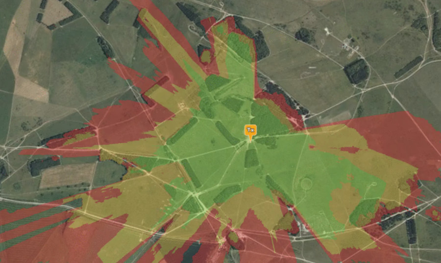
Best Site Analysis (BSA) is a monte-carlo analysis technique across a wide area of interest to identify the best locations for a transmitter. This can be done quickly with a new /bsa API call. The output will identify optimal sites, and just as important, inefficient sites.
This feature is powerful for IoT gateway placement, 5G deployments and ad-hoc networking where the best site might presently be determined by a map study based on contours as opposed to a LiDAR model.
Best Site Analysis
High speed
Our GPU engine is up to 50 times faster through the API than the current (CPU) engine SLEIPNIRTM
By harnessing the power of high performance graphics cards, we are able to complete high resolution LiDAR plots in near real time, negating the need for a “go” button, or even a progress bar. This speed enables API integration with vehicles and robots which will need to model wireless propagation quickly to make better decisions, especially when they’re off the grid. It was designed around consumer grade cards like the GeForce series but supports enterprise Tesla grade cards due to our card agnostic design.
Economical
Our implementation is efficient by design. We want speed to model wireless coverage but not if it requires kilowatts of power. During testing we worked with older GeForce consumer cards and were able to model millions of points in several milliseconds with less than 50W of power. Or in other words, the same power as flicking a light bulb on and off.
Any fool can buy large cards and waste electricity, but we’re proud to have a solution which is fast and economical. This also means it can be run on a laptop as it’s available now as our SOOTHSAYER product.
Open API
The GPU engine is an “engine” parameter in our /area API so you can use it from any interface (or your own custom interface) by setting the engine option in the request body. The OpenAPI 3.0 compliant API returns JSON which contains a PNG image so for existing API integrations using our PNG layers there will be no code changes required to enable it.
Self-hosted GPU server
Instead of buying milk every month you can buy the cow. We also sell SOOTHSAYER which is a self-hosted server with our GPU engine onboard. You get to use your existing LiDAR data too, so you’re not buying it twice.
In radio planning, accurate terrain data is only half the story.
The other data you need, if you want accurate results, is everything above the surface such as buildings and trees.
This is known as land cover or in radio engineering; clutter data.
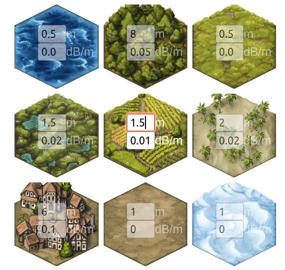
Clutter data
Clutter manager with 18 bands
In October 2021, the European Space Agency released a global 10m land cover data set called WorldCover with 9 clutter bands.
In our opinion, the ESA data is a sharp improvement on a similar ESRI/Microsoft 10m land cover data set also published this year.
The land cover can be used to enhance coarse 30m data sets to distinguish between homes and gardens, or crops and rivers. It’s space mapped so has every recent substantial building unlike community building datasets which can be patchy outside of Europe.
This data was previously very expensive. A price reflected in the eye watering pricing of legacy WindowsTM planning tools.
The data has 9 bands which have been mapped to 9 land cover codes in Cloud-RFTM. Combined with our recent 9 custom clutter bands, we have 18 unique bands of clutter which you can use simultaneously.
We have integrated the 10m data into our SLEIPNIRTM propagation engine which as of version 1.5, can work with third party and custom clutter tiles simultaneously, in different resolutions.
This is significant as it means you can have a 30m DSM base layer, enhanced with a 10m land cover layer, enriched further with a 2m building which you created yourself. Effectively this gives you a 10m global base accuracy with potential for 2m accuracy if you add custom obstacles. The interface will let you upload multiple items as a GeoJSON or KML file.
9 band custom clutterClutter menuGeoJSON clutter upload
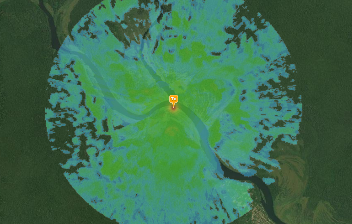
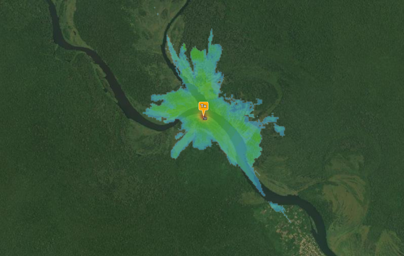
Demo 1 – The Jungle
Always a tricky environment to communicate in, and model accurately due to dense tree canopies. In this demo, a remote region of the Congo has been selected at random for a portable VHF radio on 75MHz with a 3km planning radius.
This area has 30m DSM which out of the box produces an unrealistic plot resembling undulating flat terrain. This is because the thick tree canopy is represented as hard ground and the signal is diffracting along as if it were bare earth. The result therefore is that 3km is possible in all directions.
By adding our “Tropical.clt” clutter profile, calibrated for medium height, dense trees, we get a very different view which shows the effective range through the trees to be closer to 1km, or less, with much better coverage down the river basin, due to the lack of obstructions.
VHF radio in Congo with 30m DSM30m DSM + 10m Land cover
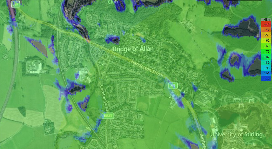
Demo 2 – A region withoutLiDAR
Scotland has very poor public LiDAR compared with England which has good coverage at 1m and 2m.
For this demo, Stirling was chosen which has 30m DSM only. A cell tower on a hill serving the town produces an optimistic view of coverage by default but when enhanced with a “Temperate.clt” clutter profile, calibrated for solid and tall town houses and pine forests (eg. > 50N, Northern Europe, Northern USA) we get a much more conservative prediction. As a bonus, the base resolution has improved three fold to 10m.
LTE site in Stirling with 30m DSM30m DSM + 10m Land cover
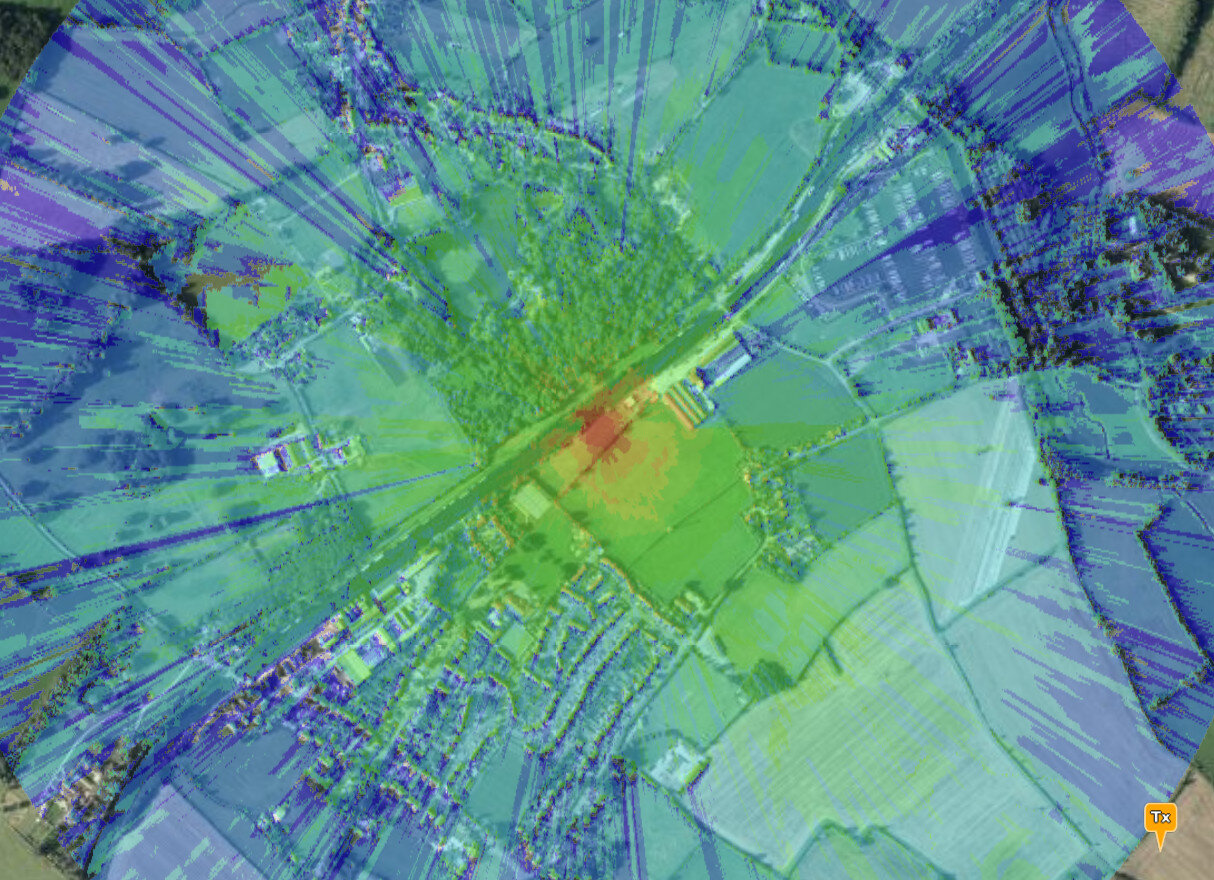
Demo 3 – A region with 2m LiDAR
You might think if you’ve got high resolution LiDAR data that’s enough. Wrong. Soft obstacles like trees especially will produce excessive diffraction as if they were spiky terrain. This manifests itself as optimistic ‘great’ coverage due to the diffraction coverage. By adding our “Temperate.clt” profile again we make trees absorb power and see where there are nulls in our coverage – beyond the houses and woods.
Despite our land cover being only 10m resolution, we are able to benefit from the full LiDAR resolution with 2m accuracy.
UHF radio with 2m LiDAR2m LiDAR + 10m Land cover
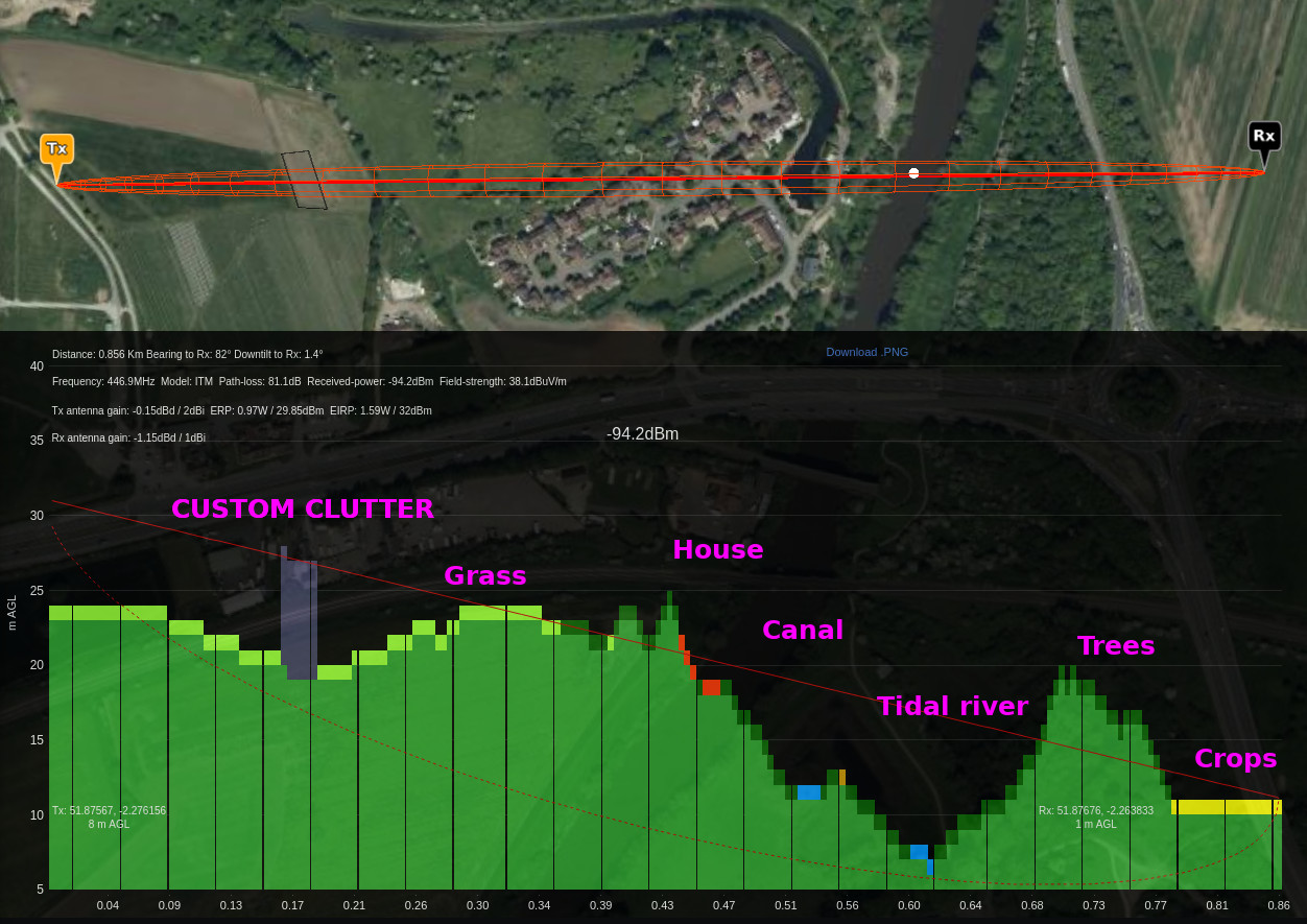
Inspecting a profile
The path profile tool will now show you colour coded land cover as well as custom clutter and 3D buildings. Crops are yellow, grass is green(!), Trees are dark green, built-up areas are red, 3D buildings are grey, water is blue…
The most significant feature in this image isn’t the coloured land cover, or the custom building (as both are features we’ve done before), or the fact we know the tidal river Severn sits lower than the man-made Canal beside it, It’s the fact that both are being used in the same model at the same time. They are different sources, different resolutions, different densities…
Path profile for 860m link showing 2m LiDAR, 10m Land cover and 2m custom building
Using and editing a profile
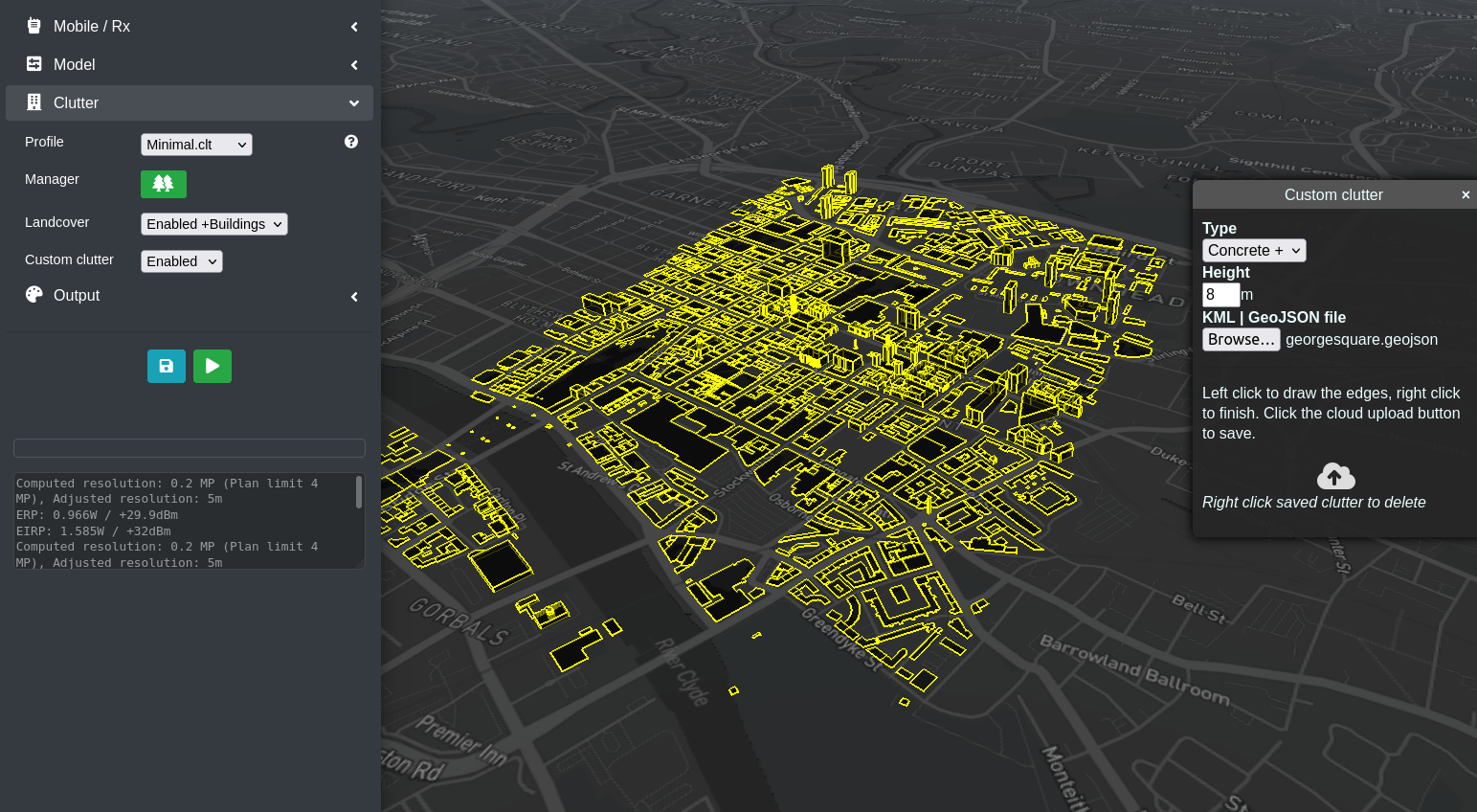
Clutter menu with 3D buildings enabled
Once you’ve got the hang of switching profiles you may find it needs optimising for your region. With the clutter manager in the web interface, premium customers can create their own profile based on field measurements for highly accurate predictions. After all no two forests or neighbourhoods are the same density.
Create your perfect profile and save it to your account. The system has 5 regional profiles ready for all users and you can add your own.
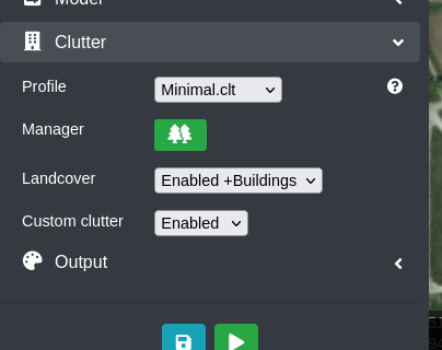
To use them, pick from the Clutter > Profile menu and ensure “Landcover” is set to “Enabled”.
If you have created custom clutter and want to use that, set Custom clutter to “Enabled” to blend it in.
We played with a few designs before settling on this very simple template method where you set a profile within the environment menu as follows. This is a new value “clt” and you can still use the existing “cll” and “clm” values to manage the system clutter and custom clutter layers.
JSON request excerpt for a temperate “European” profile, with custom clutter, with 3D buildings and a 3D building density of 0.25dB/m
Now that we have highly configurable environment profiles. it’s time to tune them with field testing. We’ve bought a heap of comms equipment and will be using it to optimise these profiles with real world measurements.
In this study we look at modelling long range microwave links and the key parameters which help get the best out of mobile microwave terminals. When sited properly, a low power microwave terminal can communicate over 100km. When sited badly the same terminal can fail to communicate 5km…
A brief history of microwave
Commercial terrestrial microwave links spread in the 1950s during post-war radio innovation and are used today as backhaul in many key public and commercial networks. A microwave station typically consists of a large tower on high ground with round parabolic dishes communicating in UHF (300MHz) bands and above. As Wi-Fi spread after the millennium, outdoor fixed wireless access (FWA) terminals for long-range (>2km) consumer wireless links became increasingly popular, especially around ISM bands, but only recently have portable tracking terminals like the AVwatch MTS become available, intended for mobile ground to air use at distances exceeding 150km.
The theory
A microwave link is designed to be high capacity and focused in order to carry a large amount of information from one point to another. For this reason they need a short wavelength so are found in UHF and SHF bands above 300MHz.
The signal has a fresnel zone around it which is sensitive to obstructions. Achieving a line-of-sight link is not a guarantee of a good connection if the fresnel zone is obstructed by trees or buildings. The size of this zone is inverse to the frequency so a higher frequency has a smaller zone, akin to a laser beam, compared with a lower frequency which has a larger zone and so requires to be higher above the earth to clear it.
Radio horizon
The maximum distance a microwave link can go over the earth has little to do with RF power and much more to do with the dish heights and the horizon which limits how far a (short wavelength) signal can go. Whilst refraction can extend a link beyond the horizon, it is variable like the weather so impractical to model accurately and in a timely fashion. A simple formula to calculate the radio horizon is 4.12 x sq(height) where height is the combined transmitter and receiver altitudes. This formula produces a table of horizons which show that an improvement in height of several meters translates to a range improvement of several kilometers due to the earth’s curvature.
Transmitter height m
Receiver height m
Radio horizon km
1
1
6
1
10
14
1
50
29
1
100
41
1
200
58
1
400
82
1
800
116
1
1600
164
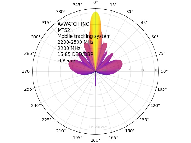
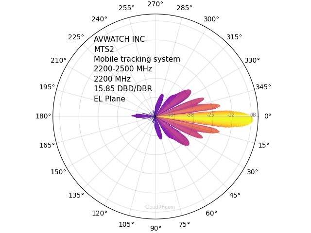
Parabolic antennas
As signal attenuation is substantial at these frequencies they require a highly directional antenna to improve forward gain and cancel noise from other angles. The larger the dish size the greater the gain and the smaller the beam.
A microwave dish antenna is easily recognised as a polar plot by it’s prominent main lobe, symmetrical side lobes and minimal back scatter. It has a very high front-to-back ratio which describes the ratio of forward power to rear in the order of +50dB. Due to it’s high directional gain it only needs to be driven with a modest amount of RF power to generate an effective radiated power of several hundred watts.
Parabolic polar plot (Azimuth)
Parabolic polar plot (Elevation)
Using and creating a directional pattern
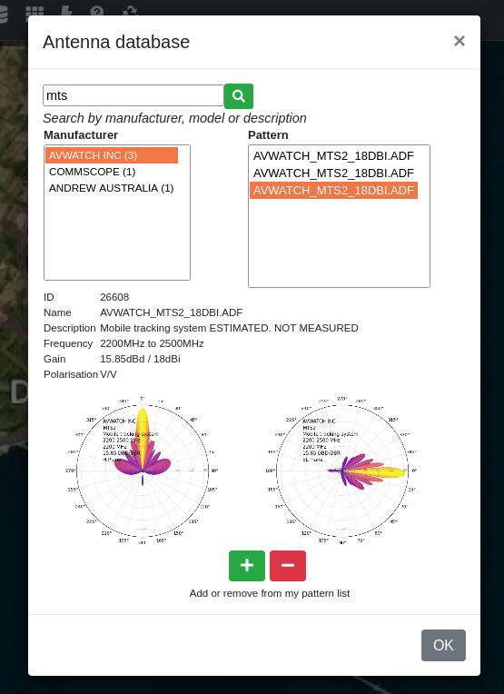
In CloudRF you can choose from thousands of crowd sourced patterns, upload your own in TIA/EIA-804-B / NSMA standards or create your own using a few parameters.
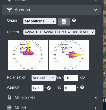
To select a template, open the Antennas menu in the web interface and click the database icon. This will open a search form. Search by manufacturer, eg. Cambium, or model. When you find a pattern you want click the green plus symbol to add it to your favourites list. You can now proceed to set the azimuth and tilt as if you were affixing it to a pole.
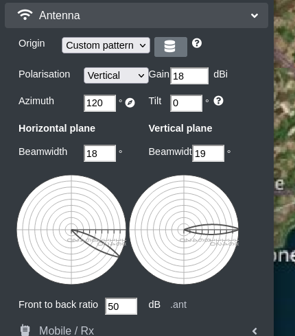
If the pattern does not exist, you can choose to use a “custom pattern” and define the horizontal and vertical beamwidths in degrees as well as the gain and front-to-back ratios in decibels to generate polar plots. These can be downloaded as a legacy .ant text file which you can upload in the service as a private pattern. A custom pattern is quick to self-generate but lacks side lobes and the full accuracy of a detailed pattern from a manufacturer.
Antenna database
Selected antenna
An over the horizon link
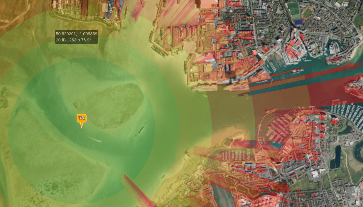
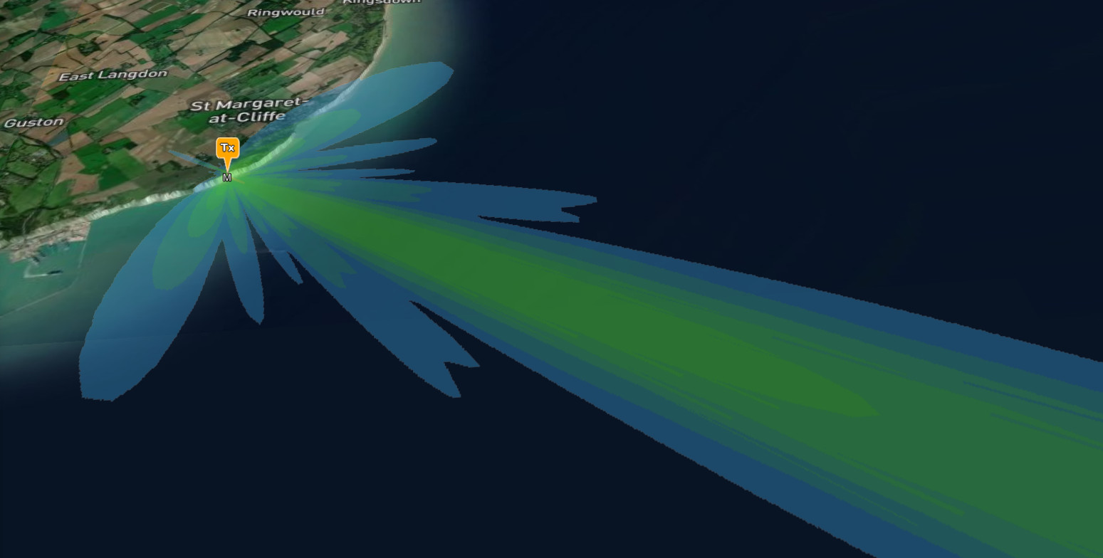
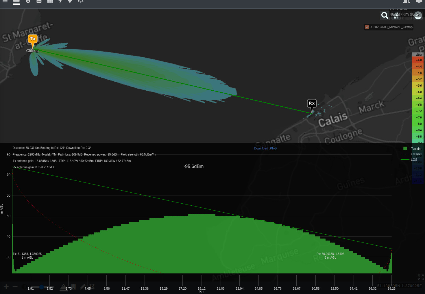
For this demo, we’re simulating a link from the cliffs of Dover in England across the English Channel to Calais, France, a distance of 40km across the sea with no obstructions. The 18dBi terminal is 1m off the ground and is using only 3 Watts / 34.7dBm power for a total effective radiated power of 189W / 52.8dBm. A receiver threshold of -100dBm was used. This is too low for high speed waveforms but would be ok for a telemetry fallback waveform like QPSK.
A bad link
With a ground receiver on top of the cliff, the link just reaches Calais. It is obstructed on the radio horizon at ~25km, a full 10km before the coastline but the height advantage of the cliff makes line of sight just possible to some parts of the town. Despite just achieving line of sight, this link would still be unsuitable due to the majority of the fresnel zone being obstructed.
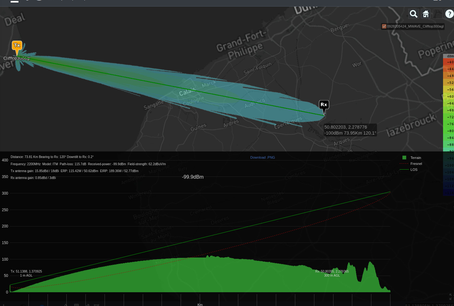
A good link
With the same cliff top terminal and RF parameters, the distant receiver is swapped for a drone 300m above the ground. The increase in height extends the link from ~25km to 75km, deep into France with good LOS.
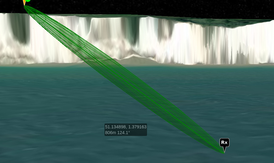
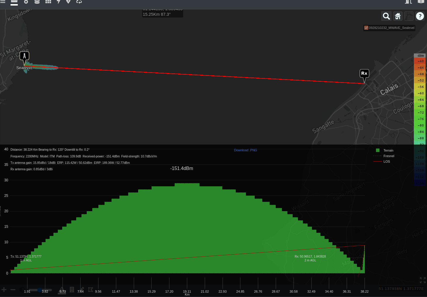
An ugly link
This time the same terminal which just achieved 75km was misused down on the beach to communicate with a small boat in the channel. It’s effective range was less than 6km due to the radio horizon. As you can see from the normalised path profile chart below, the curvature impact is substantial when the stations are on the earth!
Thresholds and modulation
The simplest way to limit the modelling is with received power measured in decibel milliwatts. In this common scale, -100dBm is a sensible threshold for most digital systems. For planning purposes, a 10dB fade margin should be added for a -90dBm threshold. The actual thresholds needed will vary by systems and waveforms. Many commercial microwave links operate very high symbol rate modulation schemas which need received power above -70dBm to function.
You can also use Bit-Error-Rate (BER) as a threshold. This unit is used in conjunction with the noise floor and the desired signal-to-noise ratio (SNR) to derive a threshold. A modulation schema like QAM64 requires a relatively high 15dB SNR compared with 5dB for QPSK which can function on weak links. These thresholds are not absolute which is why we set the desired error rate. Errors are inevitable and the relationship between the BER and SNR is best visualised as curves. If you know you want QPSK for example but are not sure what error rate to use, use a mid level error rate such as 10-3 (One bad bit for every 1000 bits) which will give you a 7dB SNR. If the local noise floor is -120dBm your equivalent receiver threshold is a pretty low -113dBm.
Conclusion
Forget RF power, height is everything in creating a successful microwave link. This might mean moving a terminal several kilometers away from the distant station in order to gain a few meters in height but the benefit will be many more kilometers in range.
We use cookies on our website to remember your preferences and repeat visits. By clicking “Accept”, you consent to the use of cookies.
This website uses cookies to improve your experience while you navigate through the website. Out of these, the cookies that are categorized as necessary are stored on your browser as they are essential for the working of basic functionalities of the website. We also use third-party cookies that help us analyze and understand how you use this website. These cookies will be stored in your browser only with your consent. You also have the option to opt-out of these cookies. But opting out of some of these cookies may affect your browsing experience.
Necessary cookies are absolutely essential for the website to function properly. This category only includes cookies that ensures basic functionalities and security features of the website. These cookies do not store any personal information.
Any cookies that may not be particularly necessary for the website to function and is used specifically to collect user personal data via analytics, ads, other embedded contents are termed as non-necessary cookies. It is mandatory to procure user consent prior to running these cookies on your website.