Author: Cameron Mickell

A common question for novice planners is which RF propagation model is best for my technology?

We have many different users employing diverse technologies, time constraints and accuracy requirements, so it is not always a quick answer but knowing about the key types of models and where to use them makes a big difference to accuracy. There isn’t a one size fits all approach to model selection for radio planning but there are definitely good defaults…

TL;DR We now recommend ITU-R P.1812 as a default model.

To help answer this question in detail, we’ve decided to explain a little about each propagation model, describe some relevant use cases and then conduct a series of measurable experiments to compare model performance and offer practical recommendations for users who need a clear starting point so they can hit the ground running with their radio planning. In this blog, we will look at model types, when to use them and how to make an educated decision on which model to use for your radio project.

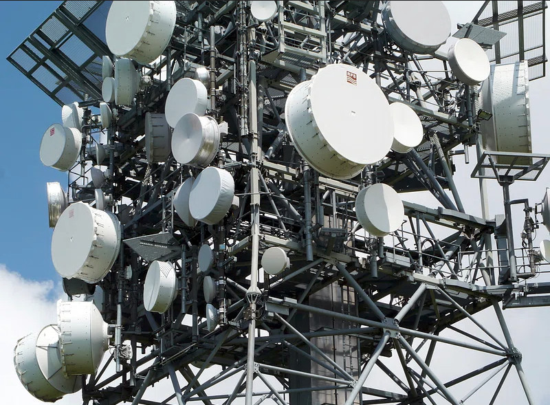
Communications Technologies across the EM spectrum

First it is important to understand there are vastly different use cases for radio technologies across the electromagnetic spectrum. Each of these technologies have their own spectrum requirements, frequency, bandwidth and power limits which have a strong influence over any potential coverage or point to point link. However, more impactful than this, is the environment and the varied ways in which they interact with radio signals.

Terrain, buildings and vegetation all interact differently with radio waves of varying frequency and different propagation models attempt to capture these behaviours in different ways. Older (1960) models pre-date developments in high resolution data so while they may adapt well to situations like their intended use, like downtown Tokyo in the case of Okumura-Hata, they will under perform in other scenarios without adjustments.

Because of this complexity, choosing the right model depends not only on your radio system but also on the environment you’re operating in. Below is a quick overview of common technologies and where they sit in the spectrum. We will look at environment latter.Communications Technologies

VHF (30–300 MHz)

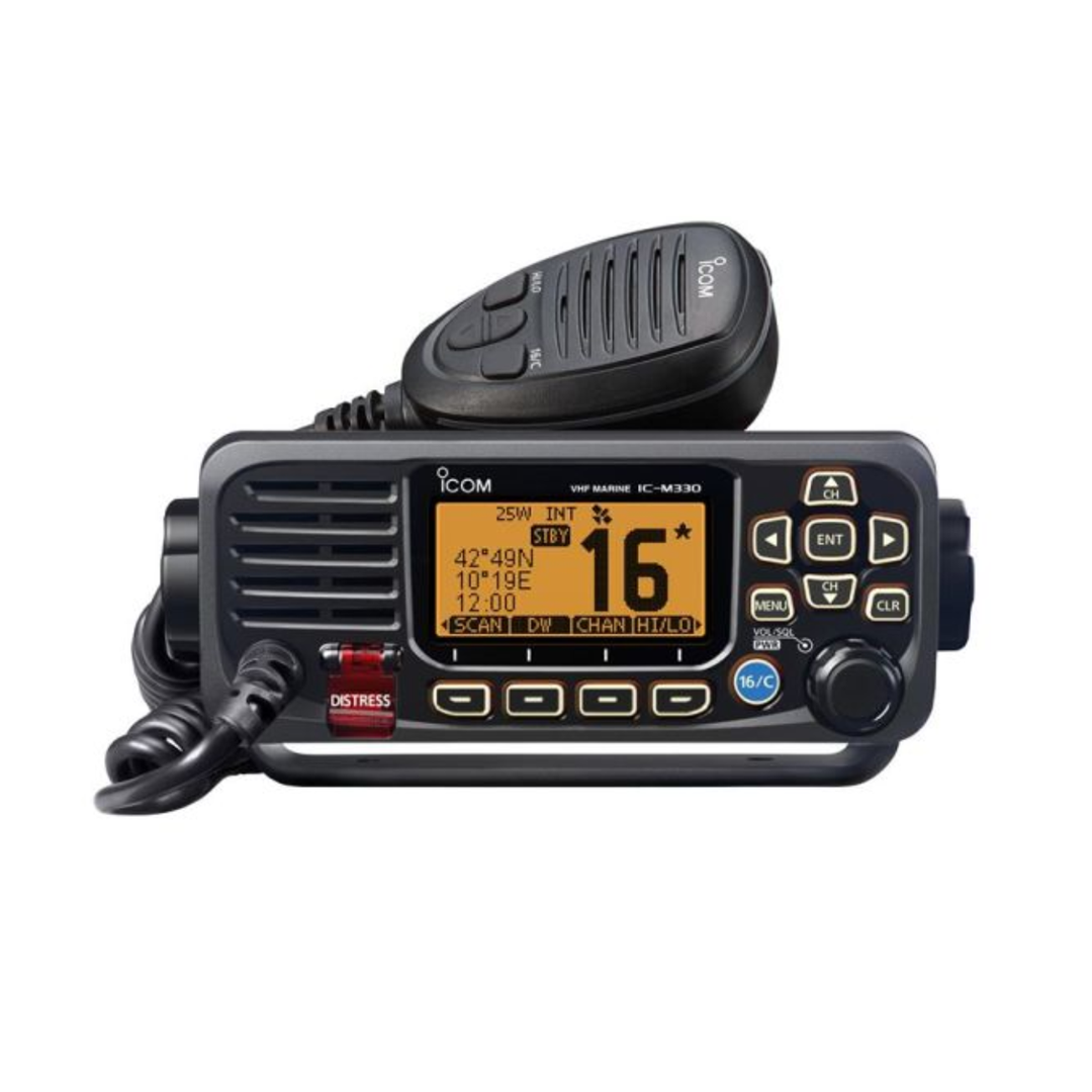
Use case: Wide area voice comms, typically extending to the radio horizon.

Propagation at VHF frequencies is highly effective over long distances due to strong diffraction, good performance over undulating terrain, and relatively low attenuation through vegetation. These characteristics make VHF particularly well-suited to wide area narrow band voice networks and maritime or land mobile radio.

VHF applications can cover both broadcast and two-way communications with the former having significantly bigger antennas mast and transmission power.

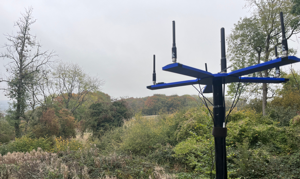
LoRa / LPWAN (433 MHz and 868 MHz EU, 915MHz US)

Use case: IoT devices, low power sensors, hobbyist networking

Propagation at these frequencies is general better through vegetation compared to higher frequencies, allowing the signals to penetrate foliage with relatively low attenuation leading to good overall range while supporting modest data rates that are well suited to low power IoT telemetry applications.

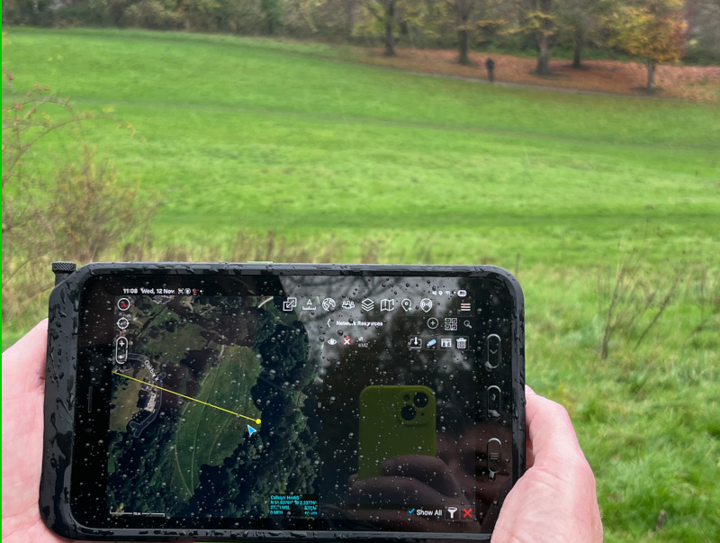
L/S Band (1–2 GHz / 2–4 GHz)

Rough equivalent: Wi-Fi, Broadcasting, Tactical radios, Microwave links

Use case: IP based networking, voice, short to medium range data links

These frequencies typically support distances up to several kilometers, depending on antenna height, power, and environmental clutter. Propagation in this range is sensitive to buildings and clutter, which limits range in dense areas but still provides reliable line-of-sight performance for short to medium distance networking. These frequencies support higher data rates than VHF or sub-GHz bands but at the expense of reduced penetration through walls and vegetation. These bands support higher data rate technologies such as Wi-Fi, video streaming or autonomous drones/robots.

LTE / 4G / 5G (700 MHz – 2.6 GHz)

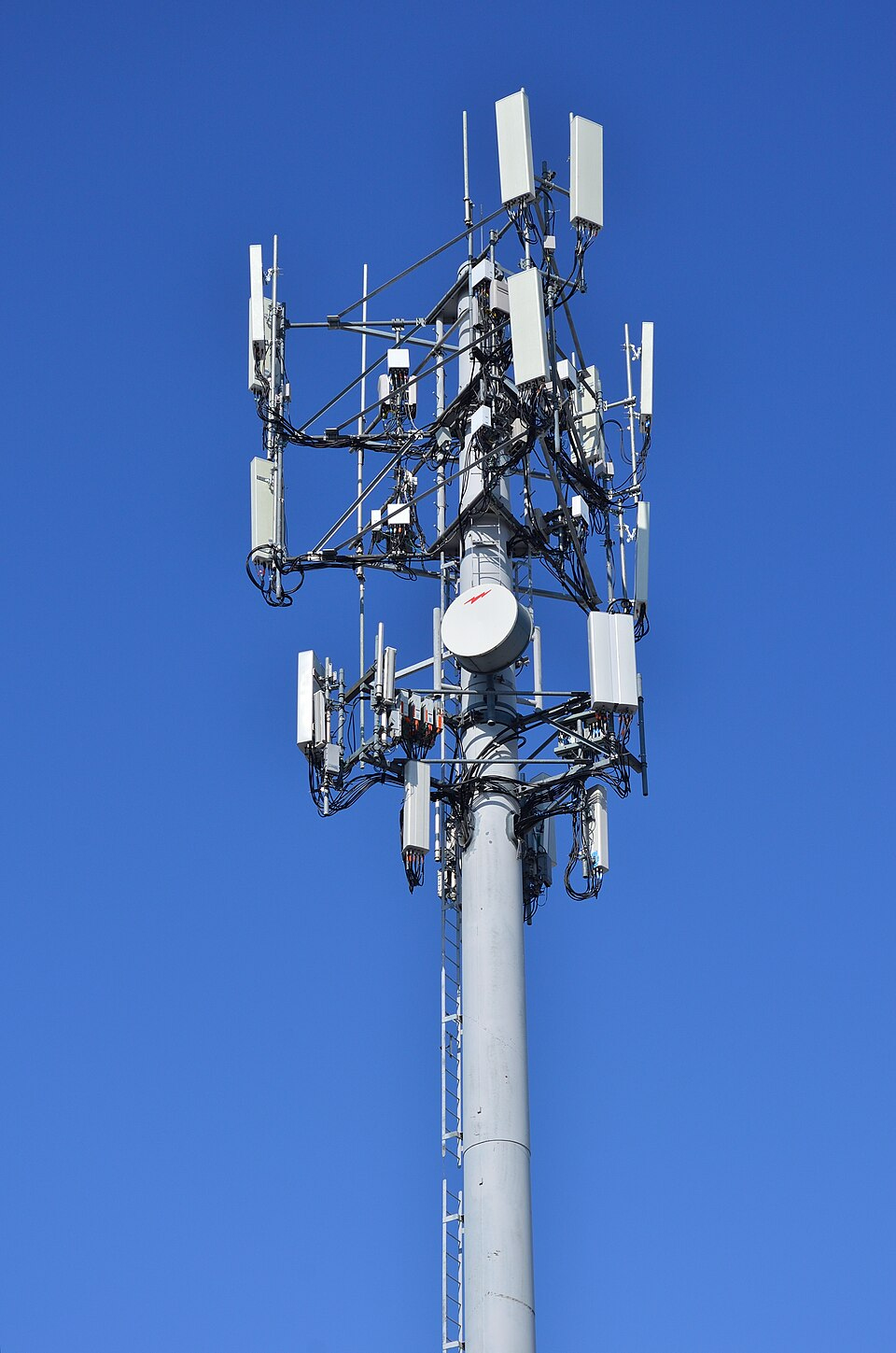
Use case: Mobile phones, tablets, broadband services

Propagation in the LTE bands offers a balanced compromise between range and capacity, allowing signals to travel several kilometres in outdoor environments while still maintaining the bandwidth needed for modern mobile broadband services.

Lower frequency LTE bands propagate further and diffract more effectively over terrain, whereas higher frequency bands are more affected by clutter and require denser cell deployments. This is why the uplink from the low power handset uses the lower bands as it has less path loss.

Because of this, LTE cells can have very different performance characteristics around terrain and clutter which makes choosing the right propagation model important.  

Across all these technologies, the environment is a key factor in determining how far or how well you can communicate. Propagation models attempt to quantify just how much the environment is going to affect the behaviour of a signal to help engineers build out these complex communications systems.

How do Propagation Models work?

Radio Propagation Models provide mathematical formulas to give predictions for the behaviour of radio waves between two points. Typically, each model aims to estimate the path loss along a link. Through recursive testing of adjacent points, a wide area can be studied to produce a signal map.

Prediction of path loss is necessary for radio engineers and operators to create accurate link budgets and generate functional communication systems or sensors. Across all models, there are two principles:

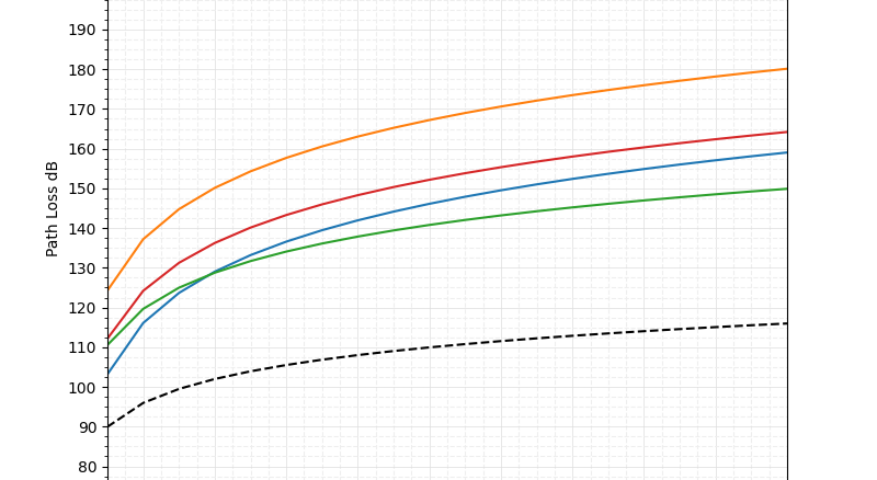
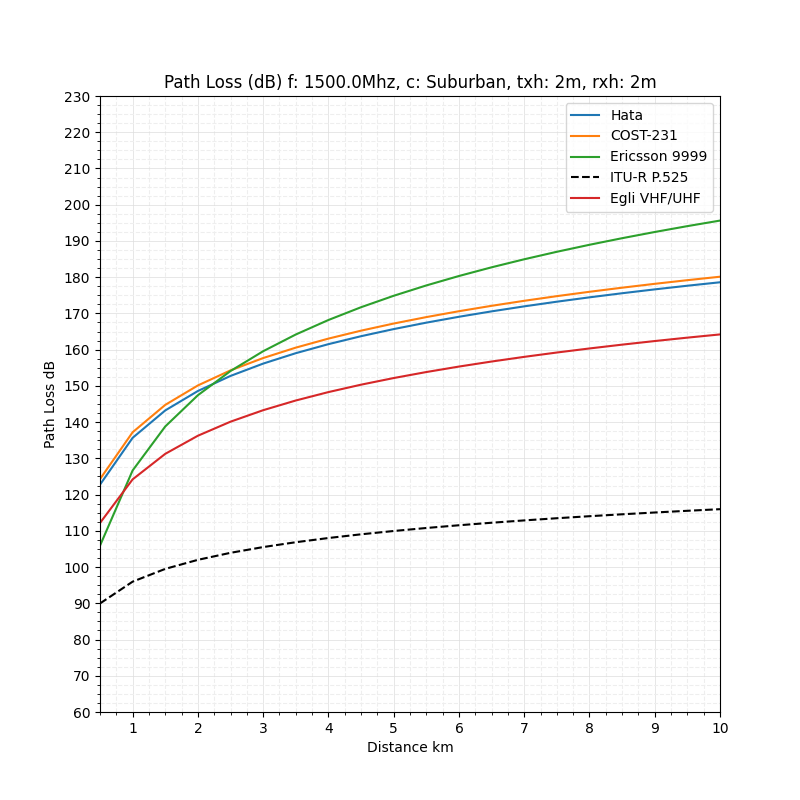
The common principle of free space loss is that path loss increases with both distance and frequency. The plotted curves below demonstrate this well.

The next principle is that each model has a unique path loss for an identical link. These curves are representative of an ideal test case of transmitting to a receiver with line of sight across uniform terrain.  

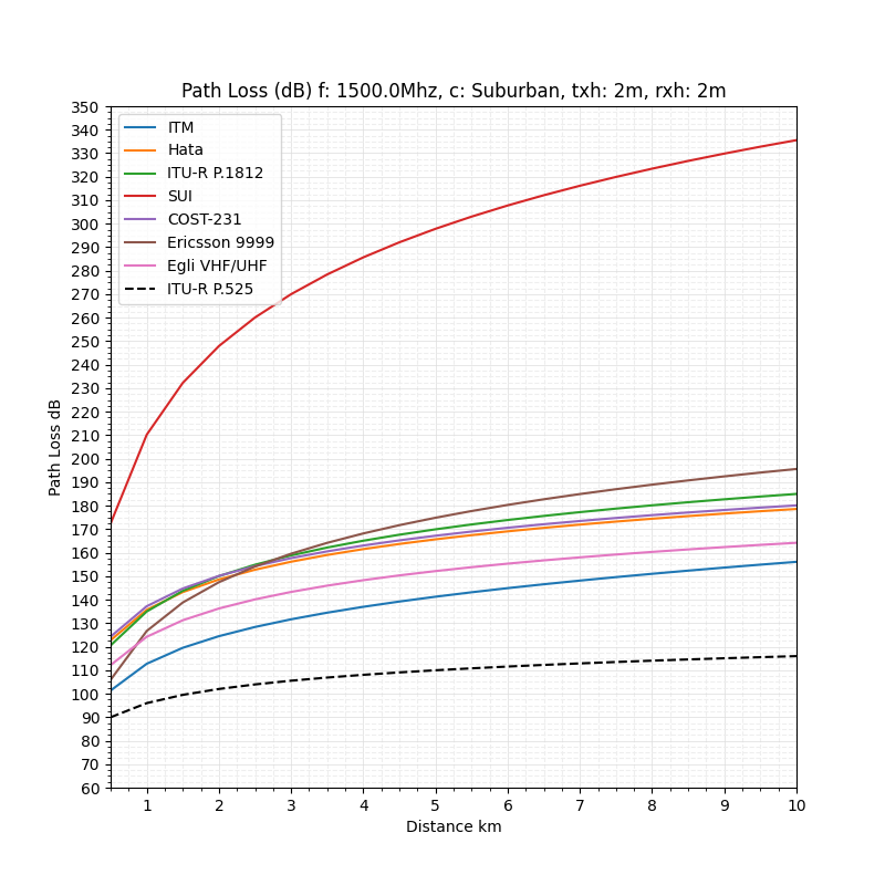
We can see different models give different results before budgeting for other sources of variation. In order to understand why this occurs we need to look at some of the key features of a model so we know when to select each one and how they work to use them effectively.

Parts of a propagation model

Each model is essentially an attempt to solve a planning problem for a communications problem. Sometimes these are very generic problems and others are tied to a specific technology and frequency range. This gives them very different reasons for existing. Bear in mind that some pre-date consumer computing! That leads researchers past and present to look for practical solutions which can come from theory or from practice to solve a wide range of communications research problems. This has led to two main types of radio propagation models: These are deterministic and empirical models.

Deterministic Models

Deterministic models are formulas which take input variables and consistently produce the same output as to opposed to “stochastic” models which are probabilistic. Researchers derive deterministic models from first principles and other phenomena to give the best possible representation of radio wave behaviour for a given set of assumptions and inputs. Both inputs and assumptions vary from model to model due to the complexity and motivation for the model.

For planners, this means the model always treats input factors consistently. It means that accurate inputs will lead to a high degree of accuracy in the output. The opposite, stochastic models, are more commonly used in fields like finance or weather modelling where there is uncertainty around a given input or future conditions.

Empirical Models

Empirical Models are data driven,built from survey data which is refined to produce a prediction of wave behaviour built on the prior observations. The advantage of these models is that they can act as ‘black‑box’ predictors that do not require describing the internal physics of the system yet still producing outputs that fit observed conditions.

The risk of using an empirical model is if it was made from tower data in a Japanese city and you use it with handheld radios in a desert, it will not perform well at all.

Input Parameters

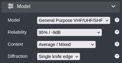
For both types of models, there are assumed input parameters that planners need to choose for a model to be applicable for their use case. For users, it is often unclear what each setting controls or how to choose an appropriate context

While propagation models provide the mathematical basis for predicting radio performance, their accuracy is ultimately constrained by the quality of the environmental data fed into them. 

Even the most sophisticated model cannot compensate for incomplete or low‑resolution terrain and clutter inputs. This makes environmental data one of the biggest contributory factors in successful RF planning.

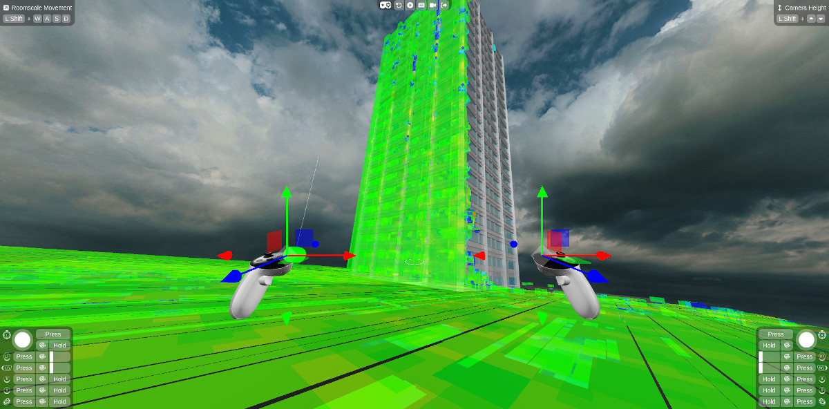
Terrain Data

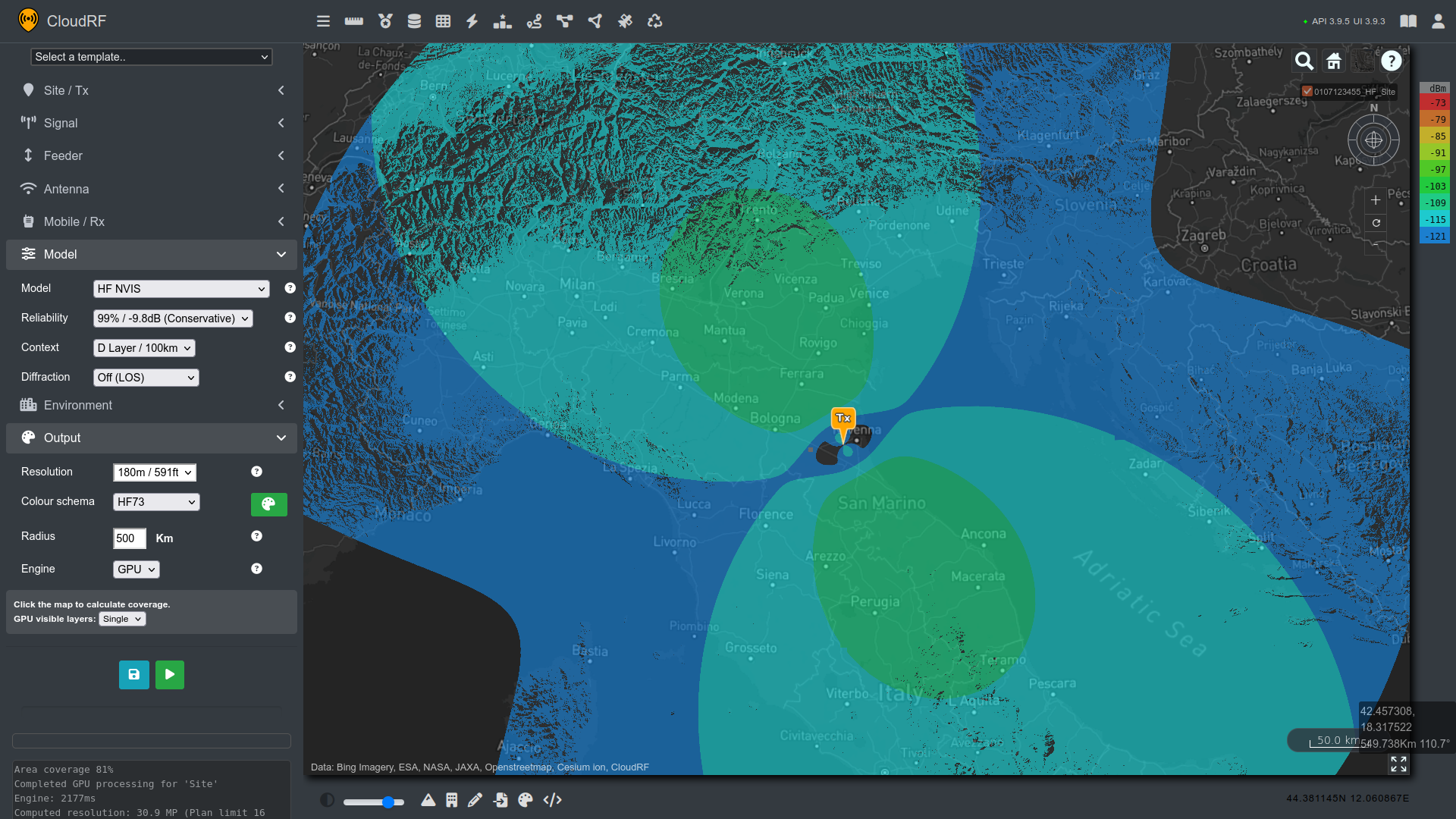
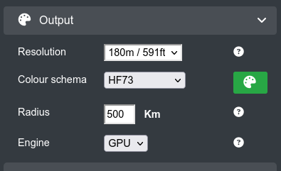
Terrain refers to the physical shape of the earth such as hills, valleys, ridges and slopes. These features directly affect radio propagation through shadowing, diffraction, and reflection. Planning tools represent terrain using tiles sized according to their chosen resolution. In CloudRF, the resolution can be adjusted from the Output section, with higher resolution leading to larger compute times, bigger output files and more accurate representation of the world.

So, when to use a certain resolution? In CloudRF there are resolutions from 1m to 300m, however key thresholds to note are 2m, 10m and 30m which map to our source data.

• 30m global datasets. Suitable for coarse planning or large areas. Limited detail often causes over‑optimistic coverage in built‑up or rugged environments. CloudRF is preloaded with 30m DSM coverage for most of the globe up to 60N with additional high latitude data for Scandinavia and Alaska.
• 10m national datasets and space based land cover (trees etc). The balance between performance and accuracy for tactical and commercial use. Well suited for coverage maps with radii up to 10s of kilometres.
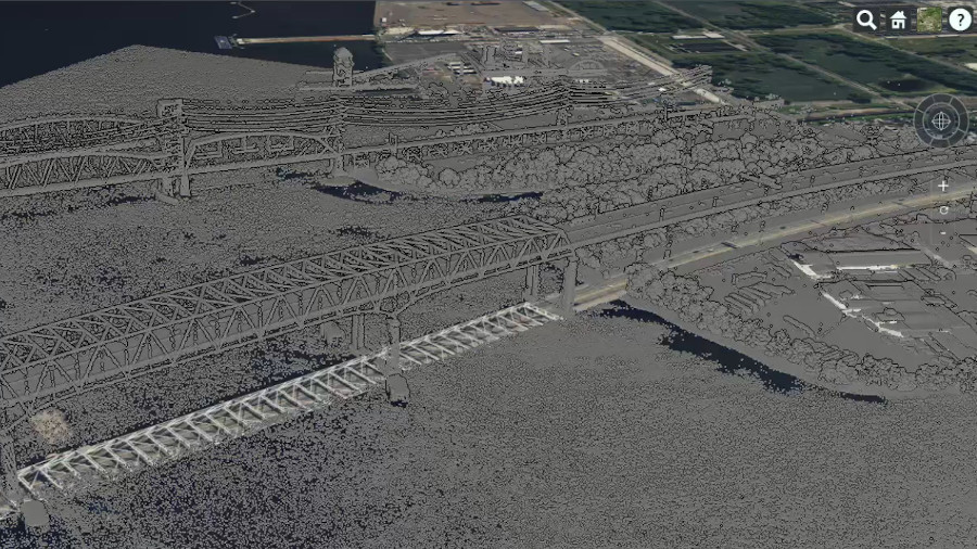
• 2m LiDAR. Highly accurate and excellent for urban, industrial or complex terrain analysis. Particularly beneficial for UHF deployments in cities or complex industrial/agricultural sites. Because most propagation issues occur when line‑of‑sight is obstructed, a high terrain resolution gives a close fit to the real environment.

Clutter Data and Contexts

Clutter describes man‑made or natural surface features that are above the terrain dataset—buildings, trees, industrial areas, bodies of water, or open ground. Different wavelengths interact with clutter in mostly predictable ways:

VHF and lower tend to penetrate vegetation more effectively but are still attenuated by dense structures. UHF, LTE and Wi‑Fi suffer greater attenuation from foliage and urban environments. LoRa and LPWAN rely heavily on clutter accuracy for predicting street‑level performance.

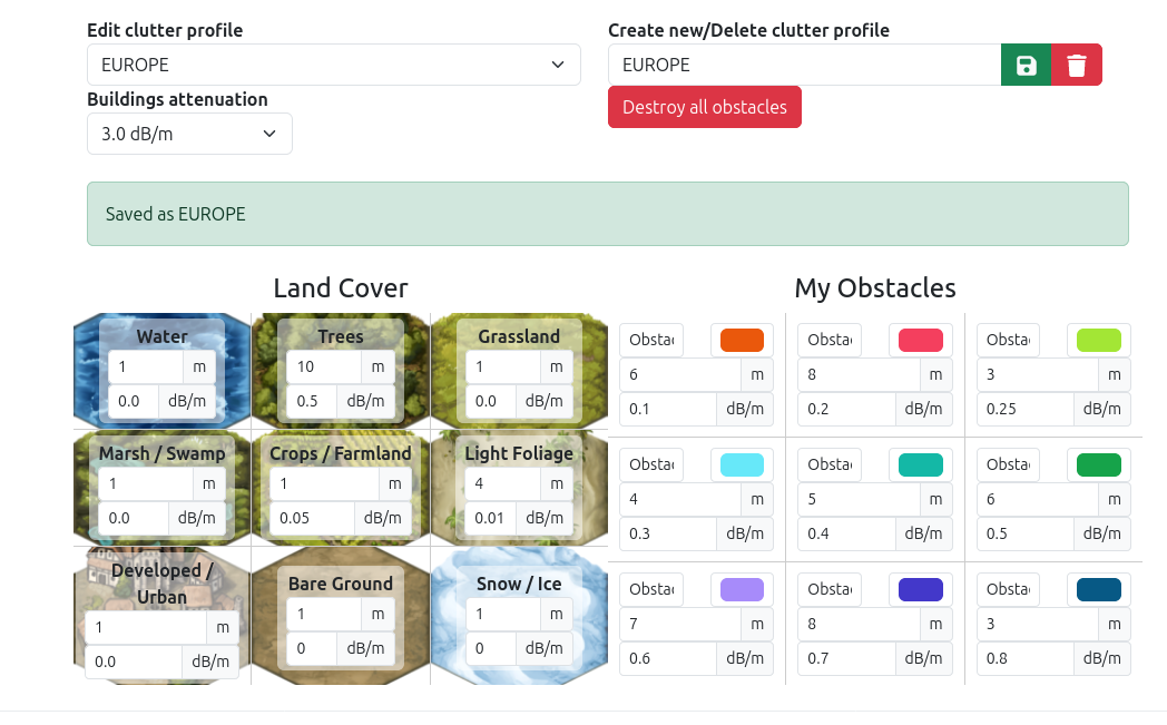
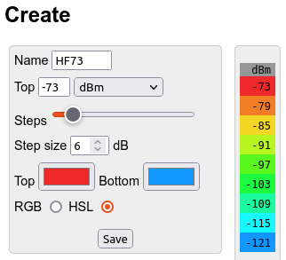
Within CloudRF, clutter is represented as classification layers with associated nominal heights and attenuation values. Selecting the correct clutter model ensures that urban and rural areas are treated appropriately, since the losses applied can vary dramatically between tree canopy, suburban housing, or high‑rise commercial zones. This allows for clutter tuning which can help with fitting survey/calibration data to a prediction.

Instead of clutter, empirical models (Okumura-Hata, COST 231 and Ericsson 9999) use contexts as factors to help tune their attenuation to an environment. These contexts are fixed empirical curves intended to represent the average path loss for a typical environment. These contexts are urban, mixed (suburban) and unobstructed (open ground). Because of this they will often not be terrain aware and in our experience do not adapt well to real clutter. The graphs below show how contexts can vary pathloss in ways that aren’t always intuitive.

Now we know what kinds of inputs our models are expecting, it is worth understanding the differences with the models available on CloudRF.

Model Bios

Irregular Terrain Model (Longley-Rice) 

The Longley-Rice model is an old but trusty general-purpose model developed to meet the needs of television broadcasting during the 1960s. As such, its input parameters have a focus on longer range high-low use cases. The model is named for its ability to account for terrain variations along the signal path. Naturally, ITM requires quality terrain data to achieve best performance. It can be used from 20MHz to 20GHz and has a range of 1-2000km for Antennas 0.5m to 3km in height.

ITU–R P.1812

The P.1812 model covers VHF and UHF bands and is recommended by the ITU since 2007 for terrestrial point‑to‑area services. The model incorporates Bullington multi-obstacle diffraction and is effective from 30 MHz to 3 GHz, making it well suited for modern commercial wireless technologies. Like the ITM, it factors in changes in terrain and incorporates clutter data into its calculations allowing it to perform very well when supplied with high quality terrain and clutter data.

General Purpose

The General-Purpose model on CloudRF is the ITU-R P.525-2 model with an additional 20dB of attenuation. The P.525-2 model is the ITU recommended free space attenuation model. It can be used across all RF frequencies from VHF up into 100GHz. With accurate clutter and land cover data, this model can be tuned to achieve single digit variation from field measurements in rural or suburban environments.  It is well suited to signals where both ends of a link are at ground level, like portable radio networks. This is outside of the comfort zone of typical high-low cellular models.

Okumura-Hata

The Okumura-Hata model is used for path loss prediction in urban environments. It is empirically derived and suitable for use around urban environments.

It assumes that the transmitter is much higher than the receiver. Specifically, 30m- 200m transmitter and 1-10m receiver heights for 1-20km. The frequency range of the original model is 150MHz – 1.5 GHz. These assumptions and range make this model best suited for cellular or broadcast environments. It uses an environment context to set its attenuation.

COST 231-Hata

This model is a popular extension of the Okumura-Hata model which brings the upper frequency to 2 GHz. COST (COopération européenne dans le domaine de la recherche Scientifique et Technique) began the Action 231 project to address the need to accurately model 2G mobile systems like GSM around 1995-1999. It was based data collected from multiple European cities to tune the model for urban environments. Because of this, it is best used in 1500-2000MHz range where the user is looking to model dynamic urban environments where LOS is often obstructed. Like the Okumura-Hata, it uses environmental contexts to be tune its attenuation.

Ericsson 9999

Ericsson extended the Hata model to 1900 MHz with special attention to the 4G and LTE use case in urban environments. Like the COST and Hata models, it’s environmental parameters can be adjusted for account for different scenarios such as rural, suburban or urban environments.

Egli VHF/UHF

The Egli model was developed by John Egli based his research with the US Army Signal Corp Labs in the early 1940s. The old model is empirically derived by capturing real world path loss across irregular terrain with dispersed clutter such as trees, buildings and other structures. The model typically expects 30-300m tall base stations to a mobile station at 1.5-10m height. Egli is suitable for VHF and UHF high-low cases below 1.5GHz. Unlike other empirical models on this list, it doesn’t use environmental contexts, so it is best suited for open rural settings.

Model Bios Quick Reference Table

Model	Frequency Range	Best Environments/Use	Terrain‑Aware?	Clutter or Context Use	Strengths
Irregular Terrain Model (Longley‑Rice)	20 MHz – 20 GHz	Mixed terrain, rural, long‑range	Yes. Includes hybrid smooth earth diffraction	Use CloudRF Clutter profiles	Good for hilly/mountainous terrain; adaptable to many use cases
ITU‑R P.1812	30 MHz – 3 GHz	VHF/UHF area coverage, suburban–rural, mixed paths	Yes. Includes Delta Bullington Diffraction	Use CloudRF Clutter profiles	Excellent general‑purpose model; robust diffraction; needs accurate clutter
General Purpose	1 MHz – 100 GHz	Simple LOS, open areas, clutter‑tuned scenarios	Yes (with clutter added)	Use CloudRF Clutter profiles	Easy to use; fully wideband; predictable behaviour; optimistic without clutter.
Okumura‑Hata	150 MHz – 1.5 GHz	Urban Macro Cells	No	Urban/Suburban/Rural Contexts	Assumes high transmitter. Behaves poorly outside operating conditions.
COST‑231 Hata	1.5 GHz – 2.0 GHz	Urban Macro Cells	No	Urban/Suburban/Rural Contexts	Well validated for cities; good for obstructed LOS macro networks
Ericsson 9999	~800 MHz – 1900 MHz	Urban Macro Cells (GSM/LTE)	No	Urban/Suburban/Rural Contexts	Flexible; Needs calibration measurements; good for early LTE/GSM
Egli VHF/UHF	< 1.5 GHz	Rural VHF/UHF	No	Nil	Useful for open rural coverage; good for broadcast-like paths; assumes tall base stations;

Propagation Model Bake Off

To help us make an informed model choice, we will conduct a series of tests using real world measurements and comparing model performance to our measured data. From this we will be able to compare results across models and see well that work without diving into clutter tunning. This will lead us to the point where it is possible to make a clear recommendation on what propagation model to choose to start a project.

Defining accuracy

To grade a model, we need to understand what values indicate an accurate model. When collecting measurements from the real world, there is always a hardware measurement error. Expensive test equipment is expensive for a reason and conversely a cheap SDR is unusable for power measurements.

For our tests, we expect a measurement error around 3 dB which would represent absolute accuracy.

A score of 3 – 6 dB would indicate an excellent result, 6 – 9 dB is a good match and up to 12 dB is ok. A score higher than 12 dB would be considered an inaccurate model and/or measurements.

Both the statistical mean and the Root Mean Square (RMS) are compared. Achieving a low mean is easy enough through over fitting results but a low RMS is much harder in an urban environment as high resolution clutter must be tuned to match diverse coverage results.

We will look at 41.5MHz, 200MHz, 800MHz, 1800MHz and 2100MHz which give us a broad frequency range to test across.

VHF (41.5 & 200MHz)

VHF broadcasting is an old and difficult problem where the long range and varying terrain can disrupt line of sight to the receiver. Power ranges are significantly higher and the antennas are mounted on very tall radios.

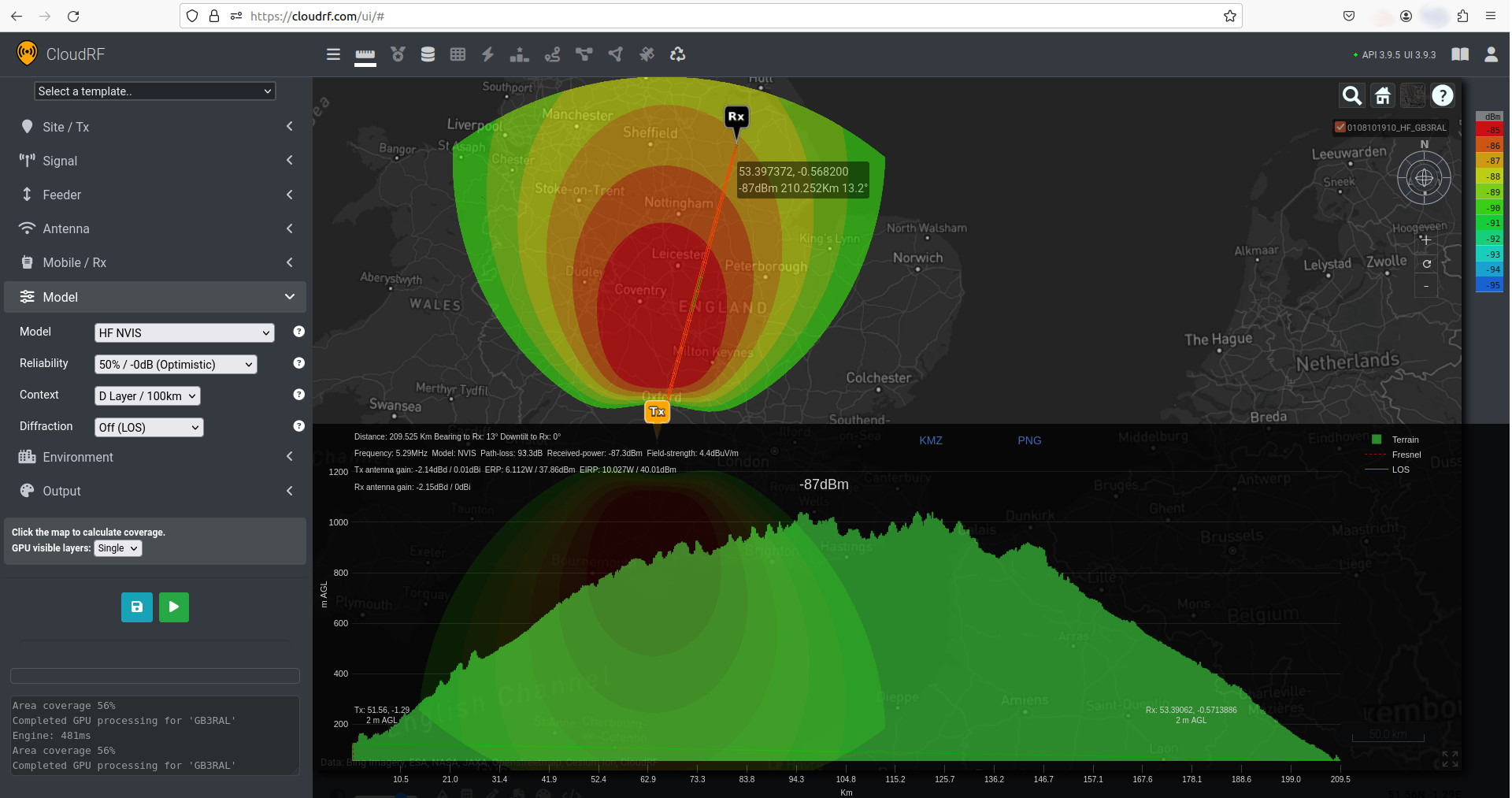
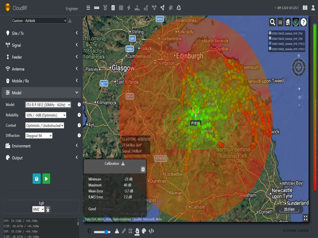
To test performance of models in the range, we referenced an ITU dataset collected by the ITU’s Study Group 3 which has a VHF broadcast data for various locations around UK, US and Europe. We will be using data from Ashkirk, Croydon and Emily Moor (41.5, 191.25, 196.25). Each area typically has over 1000 data points collected around the broadcast region, measured in field strength (dBμV). Using CloudRF, we can model expected field strength using a selection of models to see which best fits the data.

It should be noted that as this radius, terrain and clutter resolution is reduced on CloudRF due to commercial limits not present on a private server. However, as we have multiple large data sets, we can still be confident in our predictions if we see consistent performance results from case to case.

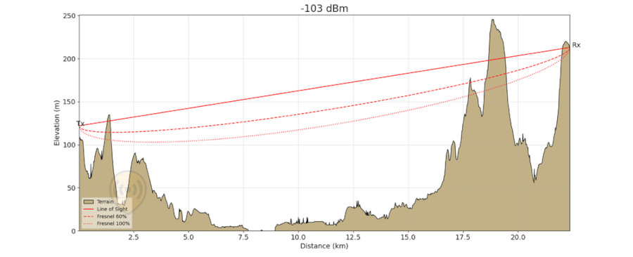
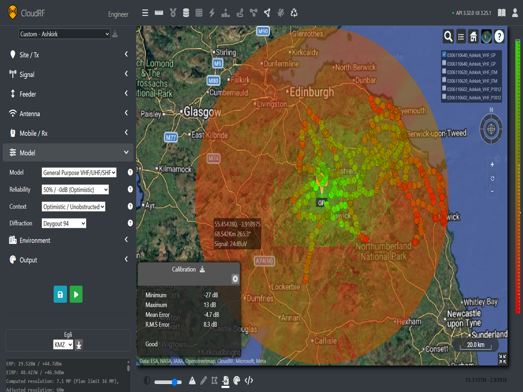
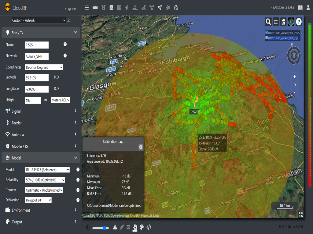
The first test involves a dataset collected from the Ashkirk broadcasting tower in Selkirkshire Scotland. The VHF antenna sits 192m above the ground, so it is very high compared to cellular or handheld radio use cases. The receive antenna is fixed at 4.3m, which will make it taller than most trees and clutter in the area. The data set contains 534 data points within an 80km radius of the tower.

Ashkirk (41.5MHz)

• ITU-R P1812 (Mean : -3.7 dB, RMS: 7.2 dB)
• General Purpose (Mean: -4.7 dB, RMS: 8.3 dB)
• ITU-R P.P525 (Mean : 9.3 dB, RMS: 11.6 dB)
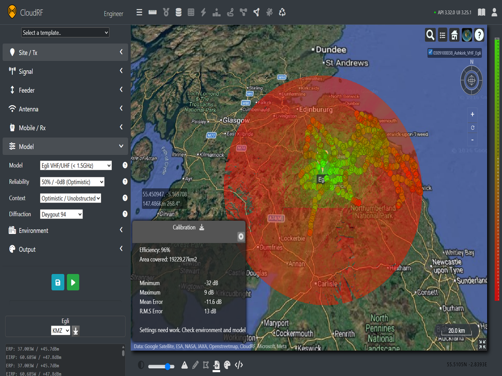
• Egli (Mean: -11.6 dB, RMS: 13 dB)
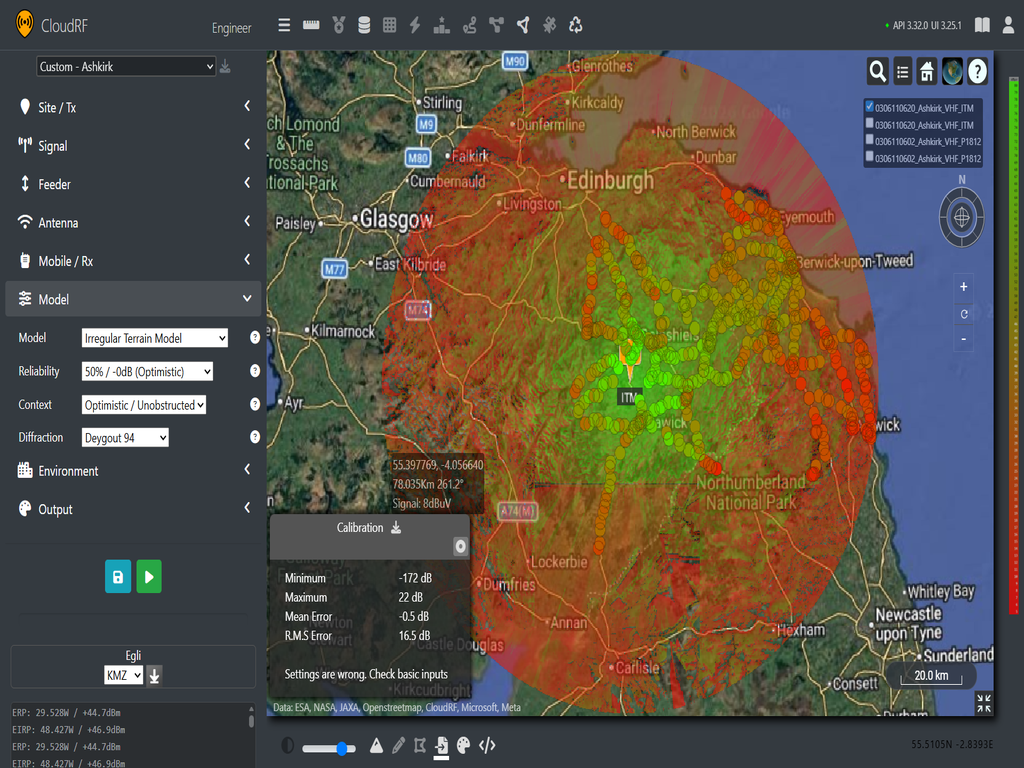
• ITM(Mean: -0.5 dB, RMS: 16.5 dB)

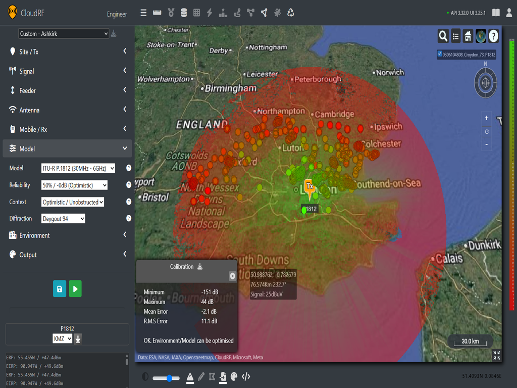
Croydon (191.25 MHz)

The second test involves a dataset collected from the Croydon transmitting station in Upper Norwood, London. The VHF antenna sits at 137m above the ground, so it is very high compared to usual use cases. The receive antenna sits at 9.8m, which places it well above most buildings and landcover expect for dense urban areas like London. The data set contains 2000 data points within a 145km radius of the tower.

• ITU-R P.1812 (Mean: -2.1 dB, RMS: 11.1 dB)
• General Purpose (Mean : -0.2 dB, RMS: 12.9 dB)
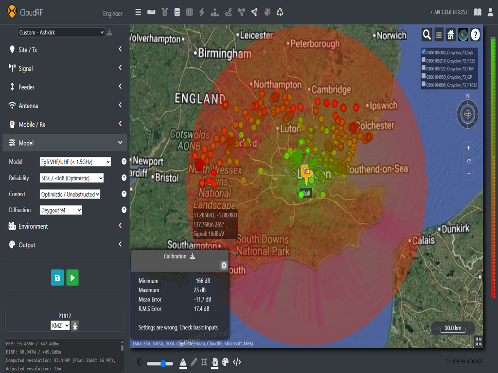
• Egli (Mean : -11.7 dB, RMS: 17.4 dB)
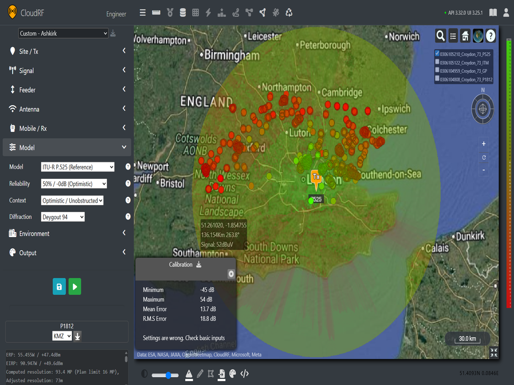
• ITU-R P.525 (Mean: 13.7 dB, RMS: 18.8 dB)
• Irregular Terrain Model (Mean error: -14.3 dB, RMS: 42.8 dB)

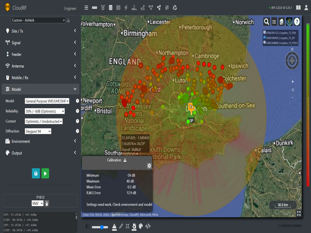
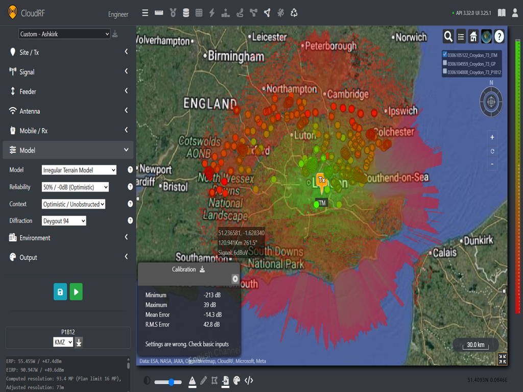
In this second test, we can see that our only acceptable prediction is P.1812 which will require further calibration to be tuned for this environment.

The third test uses data from the Emily Moor transmitter which broadcasts to the Yorkshire area. The data set contains 2000 points within a 100Km radius. The transmit height is 305m and receive height is 10m.  

Emily Moor (196.25 MHz)

• ITU-R P.1812 (Mean: -2.5 dB, RMS: 8.3 dB)
• ITM (Mean: -1 dB, RMS: 10 dB)
• ITU-R P.525 (Mean: -5.2 dB, RMS: 11.1 dB)
• Egli (Mean: 11 dB, RMS: 14.5 dB)
• General Purpose (Mean: -14.8 dB, RMS: 17.7 dB)

From our third data set we can see that P.1812 gives the best prediction again for these conditions. The significant heights involved worked against the ground based GP model but favoured ITM, developed for TV broadcasting.

VHF Conclusion

From our testing, we can see that without calibration, the models produce variable results with the test data sets. However, the one consistent exception is ITU-R-P.1812 which gives a mean measurement error of -2.76 dB with an RMS of 8.8 dB. For this range and complex environment, this is a good result which can be improved further with clutter tuning.

We can also see that our mean and root mean square values are higher than the few dB we would expect in a cellular model eg. 6dB. This is acceptable in this case as we are working over a very large area where the standard deviation of our results will increase as our resolution expands. With a large amount of diverse data points, localised errors can be diluted to establish consistent performance across data sets.

Looking at our selection of models, it is not surprising to see P.1812 outperforming the rest. Egli is a 1950 empirical model for VHF broadcasting, however it is not terrain aware so will tend to under/over attenuate through irregular terrain. Free space (P.525) will tend to be over optimistic over long distances and the added attenuation for General Purpose is better suited for handheld radios amongst clutter. So naturally, for CloudRF uses, we’d recommend starting with ITU-R P.1812 when working with VHF.

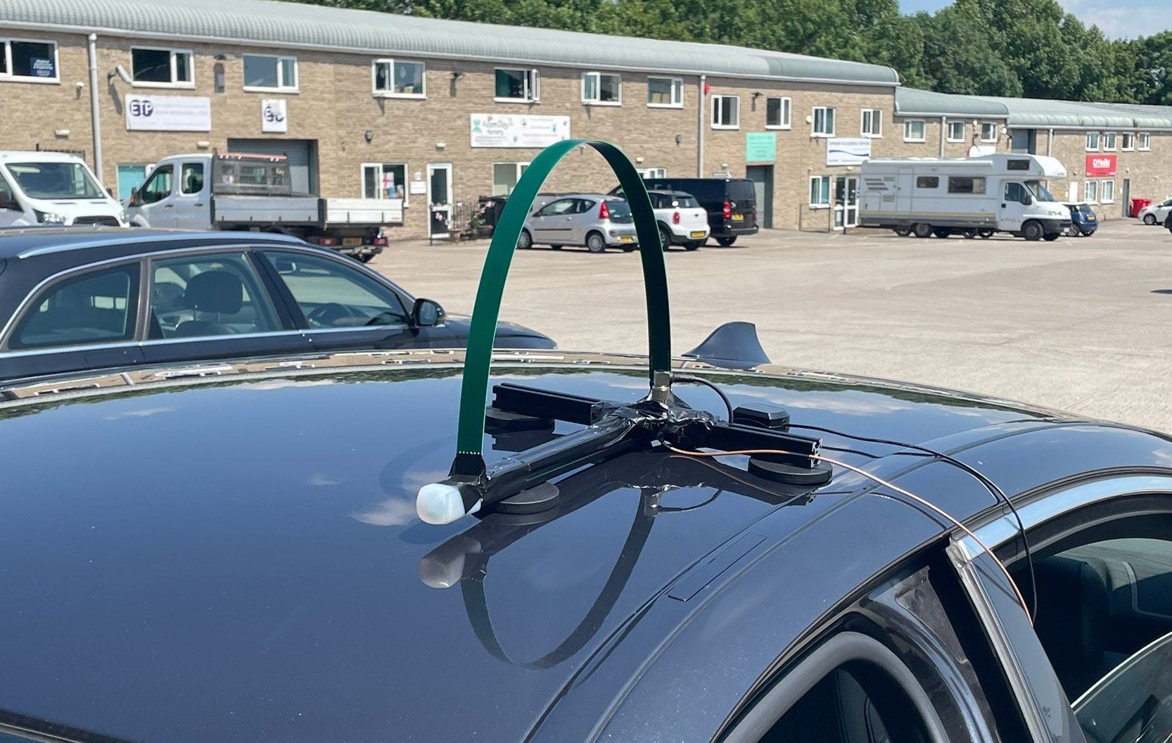
800 MHz (LoRa, UHF, Cellular)

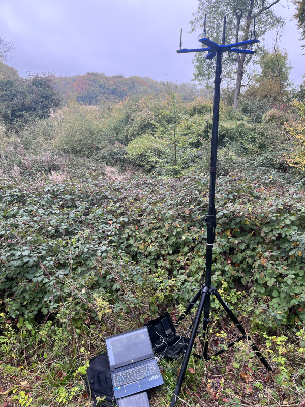
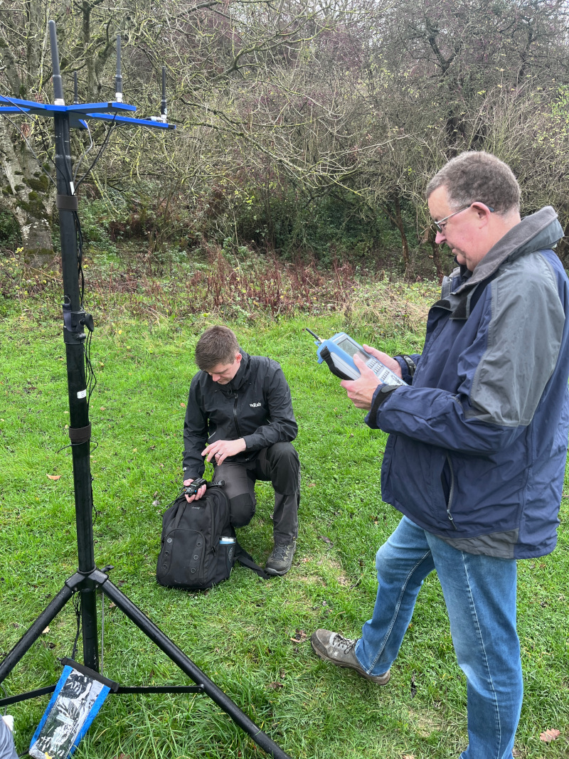
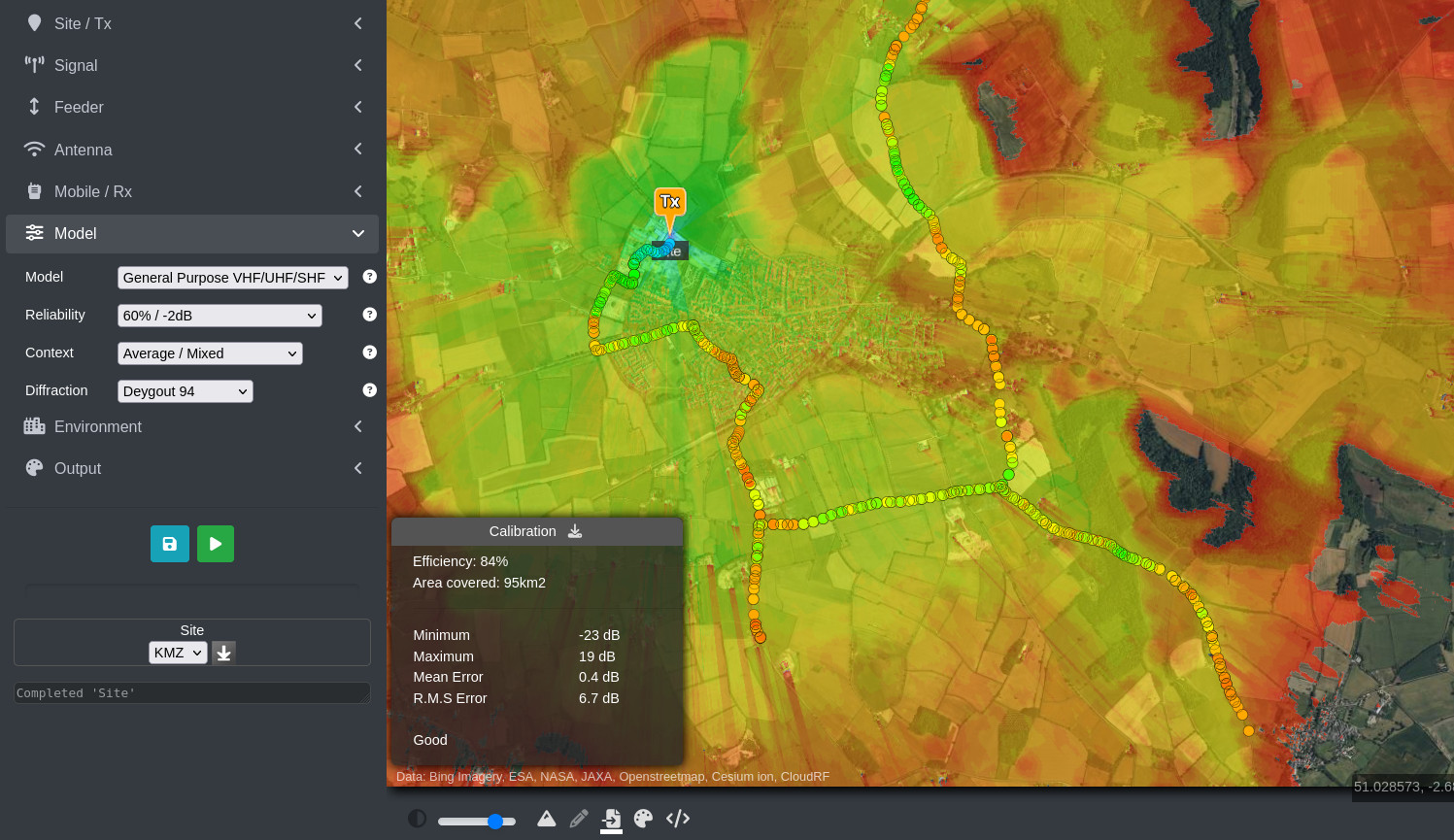
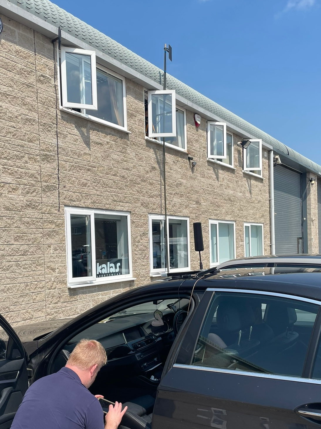
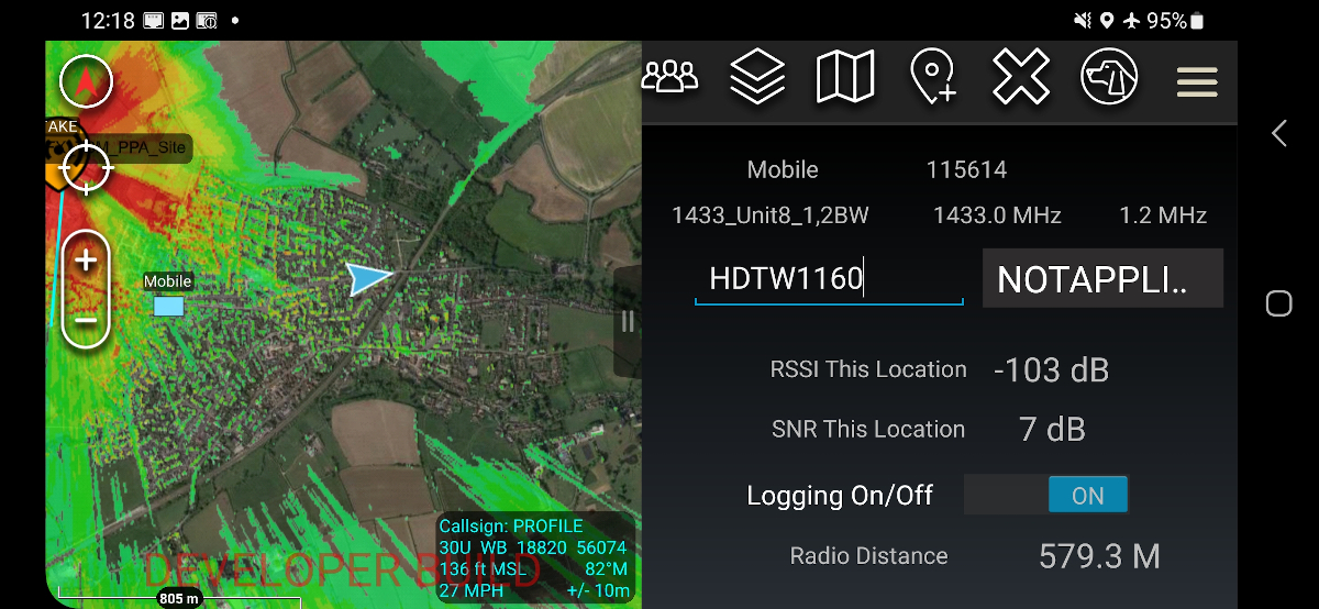
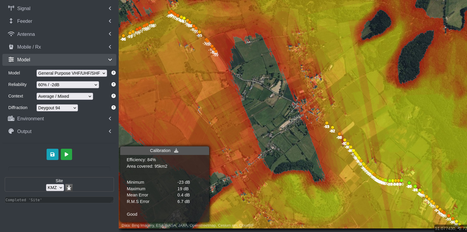
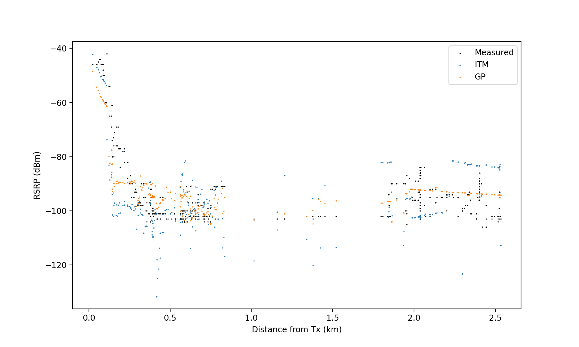
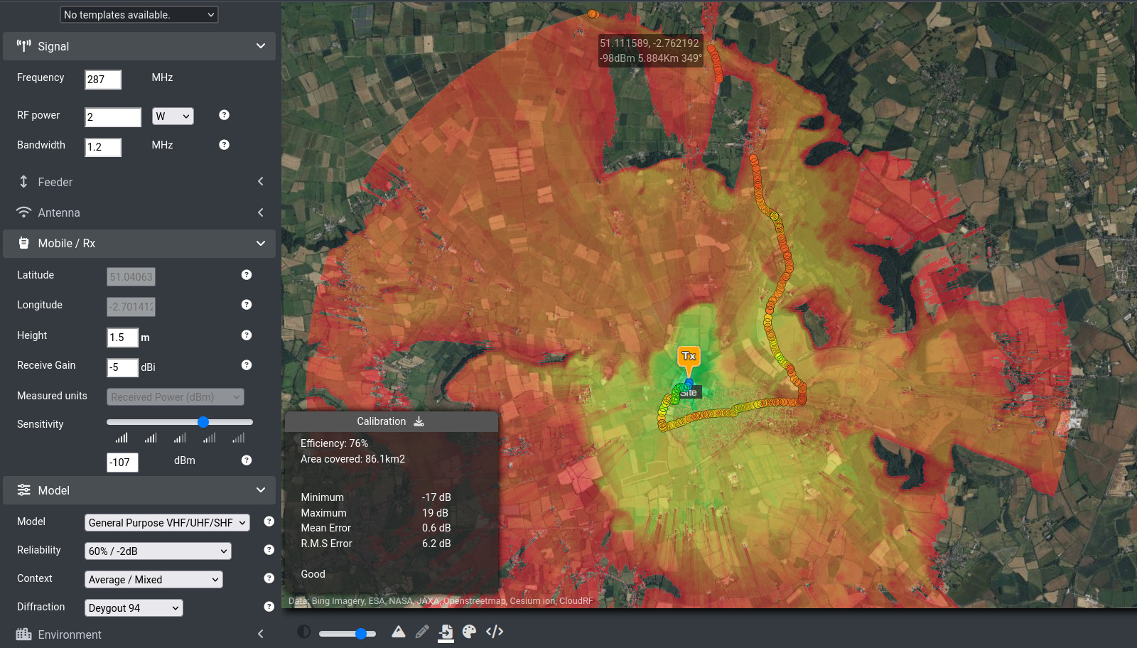
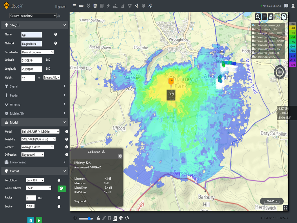
For this test, we will be using an LTE band 20 (806MHz) transmission tower with RSRP measurements taken from test handsets located with a 3 Km radius of the antenna. The Antenna itself is sitting at 12m above the ground. This serves as an excellent test of lower frequency LTE, 3G and LoRa (868MHz). Using field measurements, we will make predictions using Cloud RF and then use the calibration tool to see the average and RMS errors to see if we have a good fit between our model and our data.

The models we will test are: General Purpose, Irregular Terrain Model, ITU-R P.1812, Okuma-Hata, Ericsson 9999 and Egli. We won’t be testing COST 231 as the test data is below its intended frequency range of 1.5GHz -2GHz.

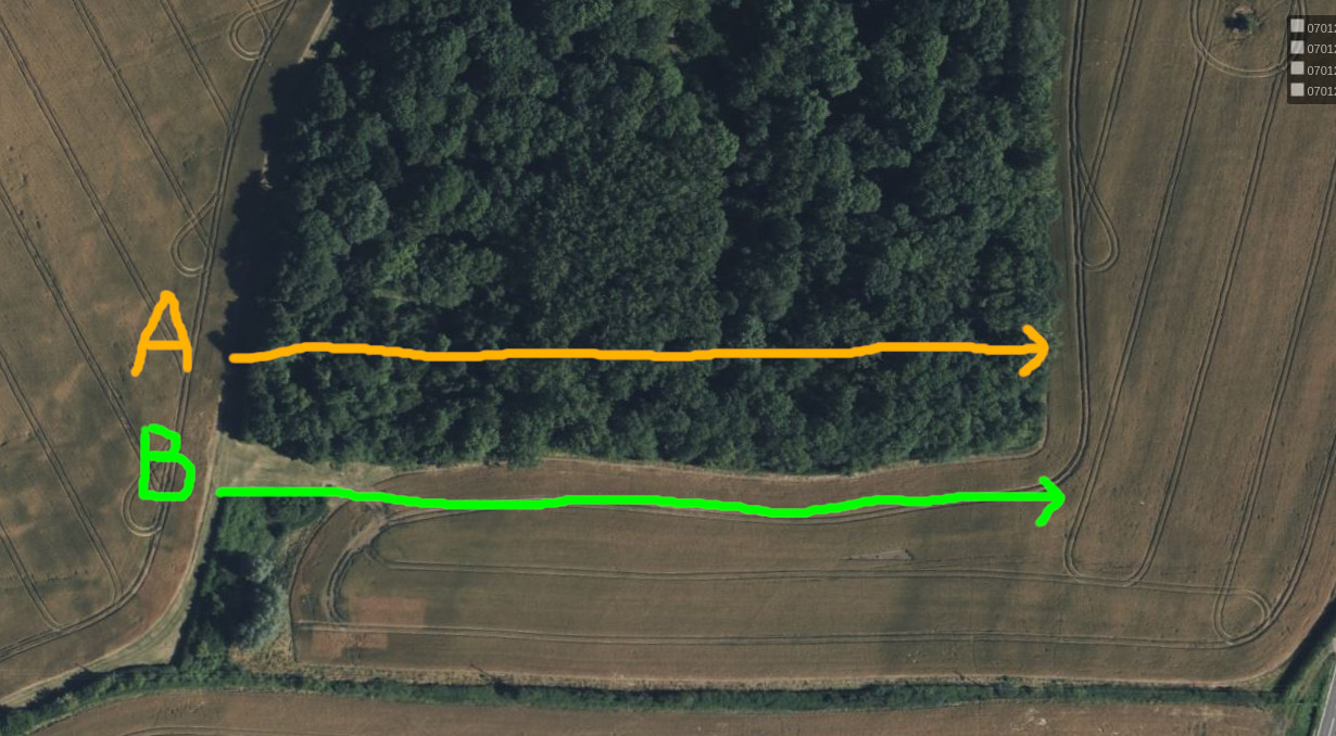
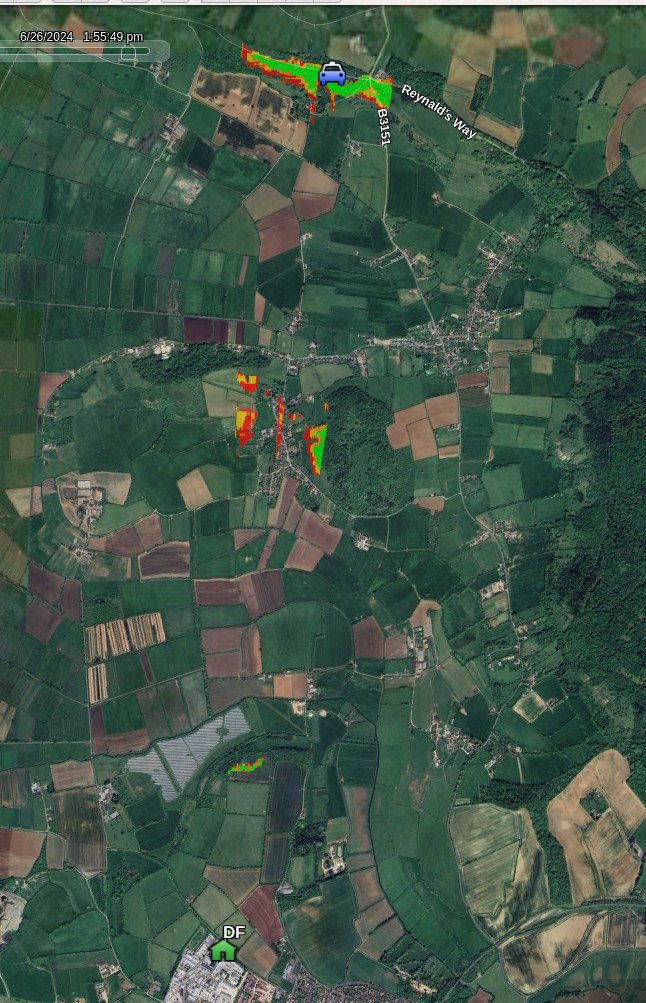
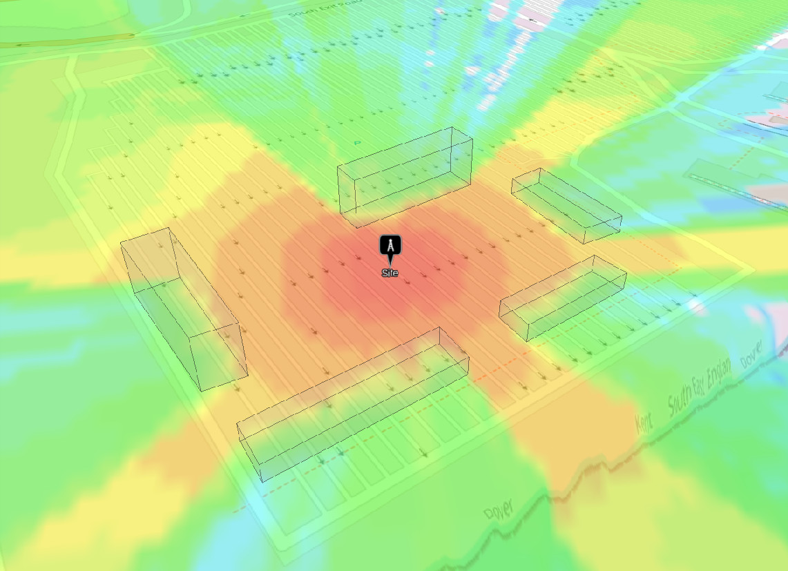
The area of interest is located to the south of the village of Wroughton, which is South of Swindon. The site sits in an open field surrounded by fields and a solar farm with good inter-visibility around the former airfield. The village of Wroughton sits to the north in the shadow of a hill, so we would expect to only see a little coverage through diffraction to the north with stronger coverage to the west, south and east being broken up by hedgerows and sparse buildings.

Wroughton (806 MHz)

• General Purpose (Mean : 2.6 dB, RMS: 3.6 dB)
• Egli (Mean : -3.4 dB, RMS: 5.7 dB)
• ITU-R P.1812 (Mean : -6.5 dB, RMS: 7.7 dB)
• Irregular Terrain Model (Mean : 12.1 dB, RMS: 12.7 dB)
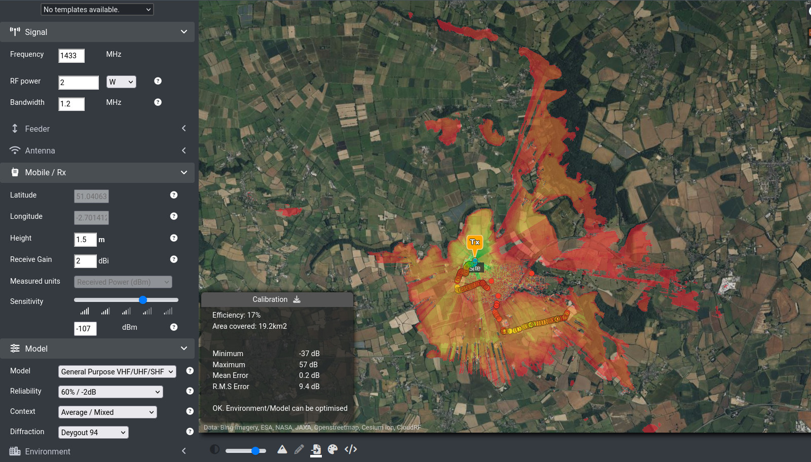
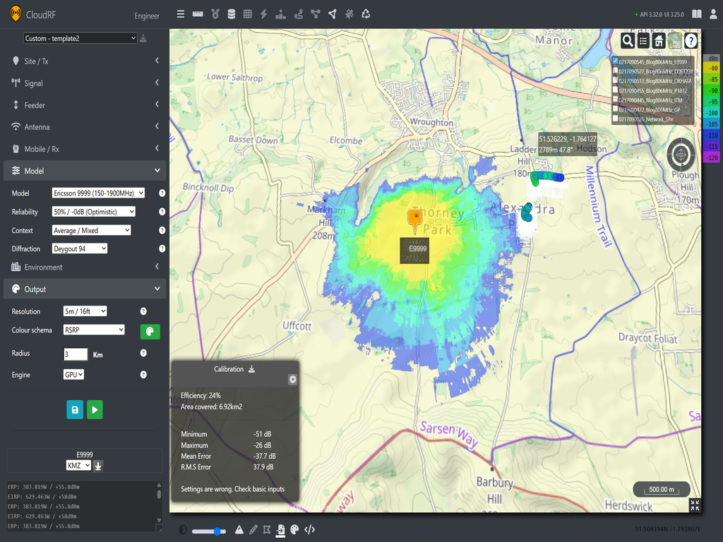
• Okumura-Hata (Mean : -37.7 dB, RMS: 37.9 dB)
• Ericsson 9999 (Mean : -37.7 dB, RMS: 37.9 dB)

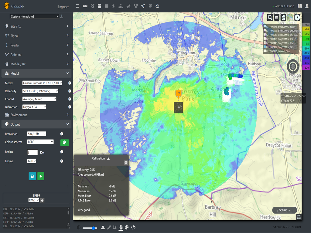
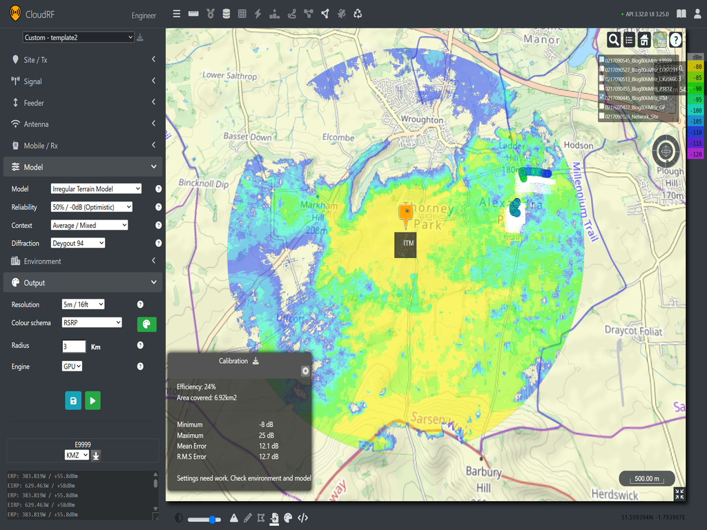
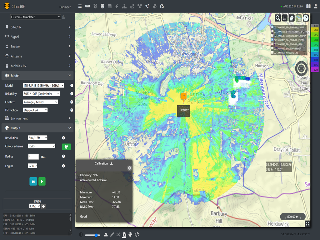
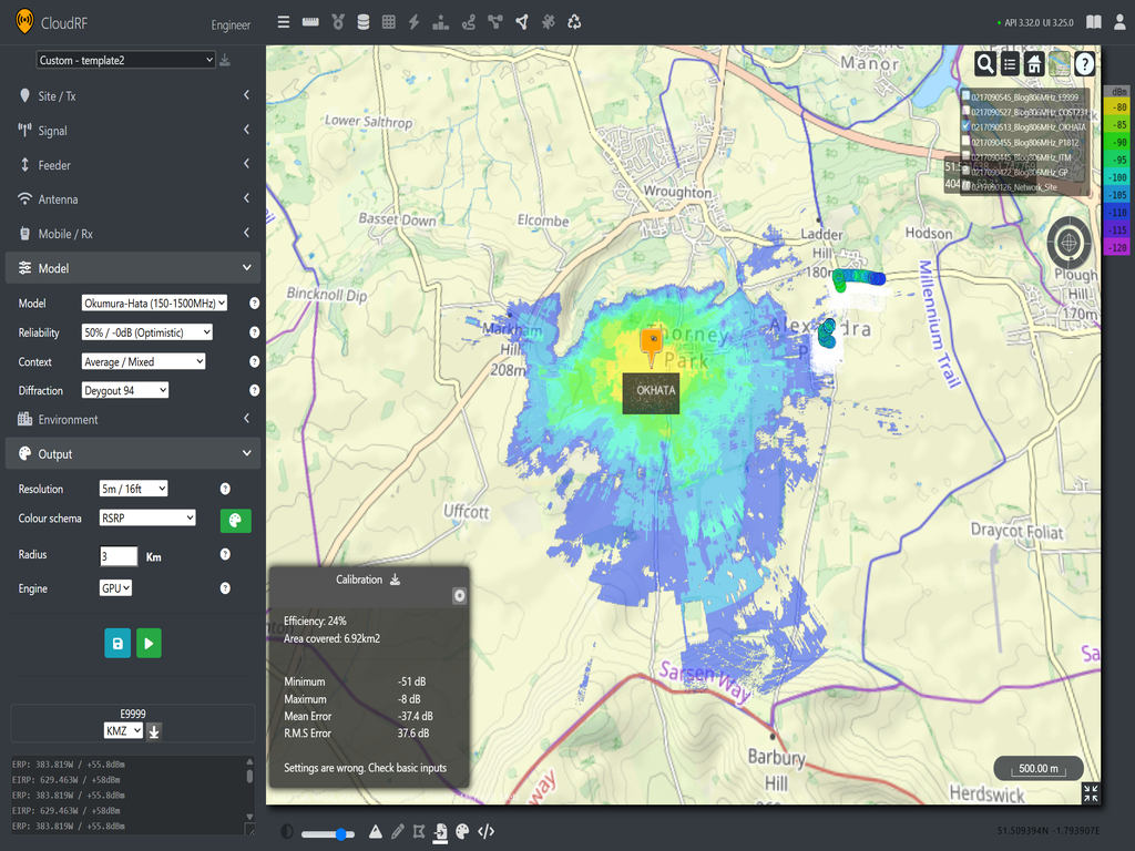
Results

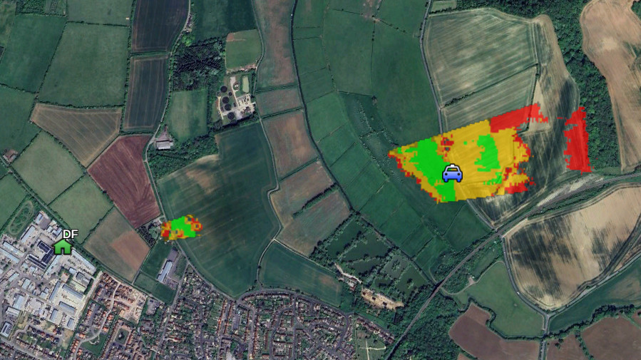
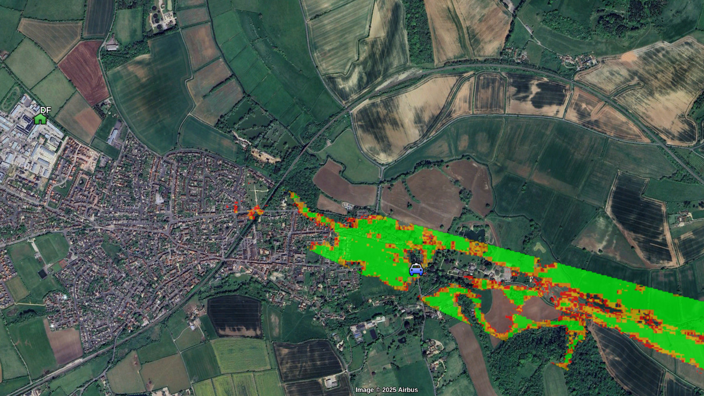
From the test, we can see that General Purpose and ITU-R P.1812 are good fits for the data, offering single digit variance. The ITM prediction is under attenuating and giving stronger coverage over similar areas to the general purpose and ITU-R P.1812. We can also see that Okumura-Hata and Ericsson 9999 are over attenuating, and we aren’t seeing coverage in the area around our readings at all.

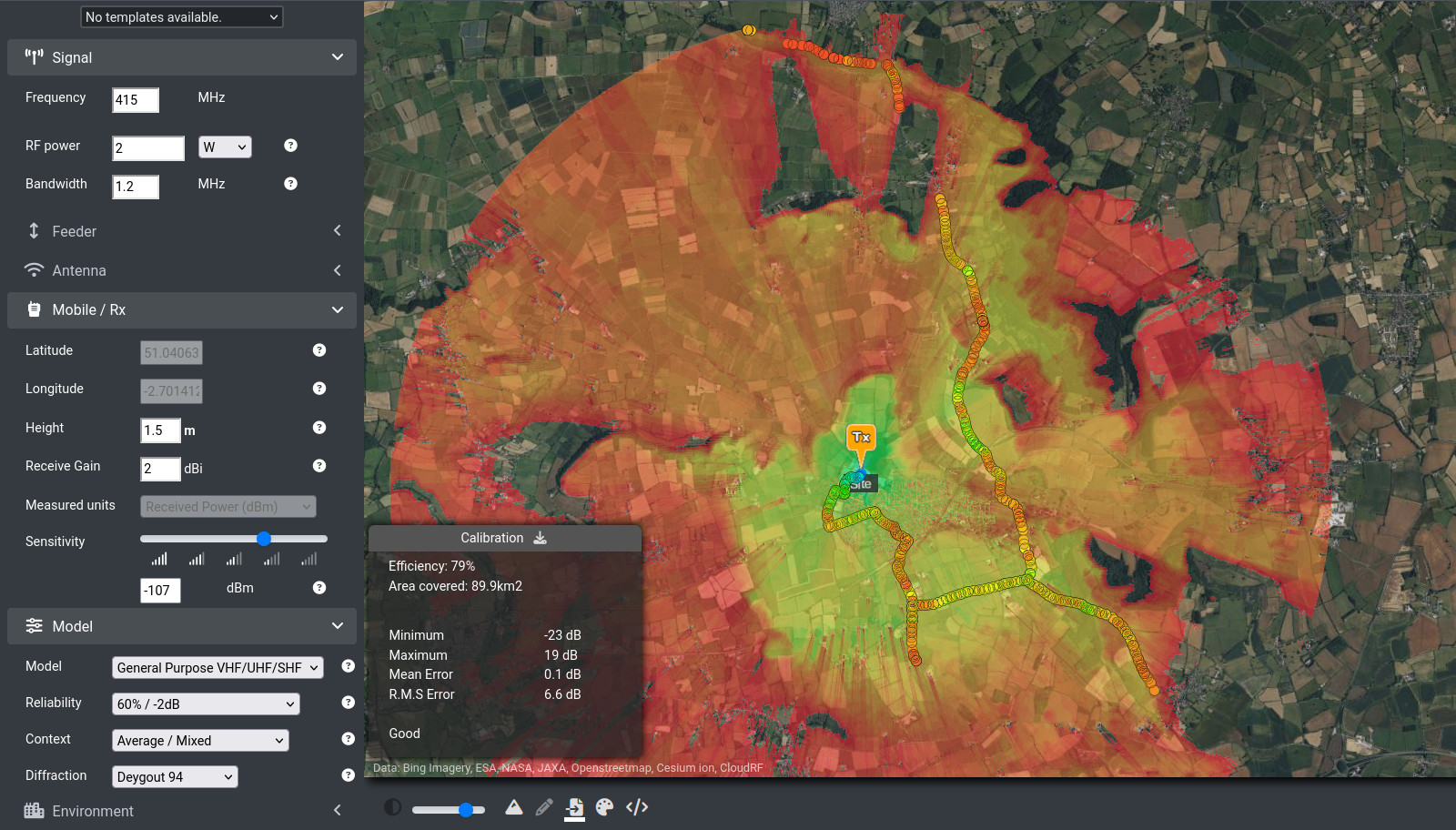
To understand these results, we can go back to their intended use cases: Okumura-Hata and Ericsson 9999 models are intended for built up urban environments and expect more obstacles and chances for diffraction. For the test template, we are using an average/mixed profile which maybe over attenuating our predictions without the environment providing enough paths for diffraction. If we look at the area of the test, we can see there is very few buildings with plenty of open fields and trees. If the context is adjusted to unobstructed, both Okumura-Hata and Ericsson 9999 should yield a better fit to our test data.

• Ericsson 9999 Unobstructed (Mean: 2.4 dB, RMS 3.5 dB)
• Okumura-Hata Unobstructed: (Mean : -6.8 dB, RMS: 7.6 dB)

By changing the context, we can see that both models now fit the data well.

UHF conclusion

CloudRF recommends ITU‑R P.1812 or General Purpose model for modelling the 800 MHz range. Our experiment supports this, demonstrating that both models provide reliable results when paired with quality clutter and land cover data.

As this test shows, empirical models such as Okumura‑Hata and Ericsson 9999 can be difficult to use without reference data because they depend heavily on selecting the correct environmental context. Without field measurements, you must rely on your interpretation of the environment to decide whether a model should be treated as urban, suburban, rural, or unobstructed. This requires time, experience, and careful reading of the model documentation especially when planning in remote or complex areas.

Deterministic models, on the other hand, have shown to perform consistently when supplied with good‑quality terrain and clutter data. As we continue conducting field tests, we are becoming increasingly confident in recommending ITU‑R P.1812 as a robust starting point for modelling LTE Band 20 (800 MHz) and similar low‑frequency systems. Because it is terrain aware and It offers good accuracy even before calibration, which makes them highly useful for time sensitive planning tasks. Additionally, as better LiDAR and DTM data becomes available, these models will increase in effectiveness as legacy empirical models become obsolete.

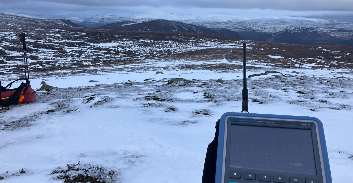
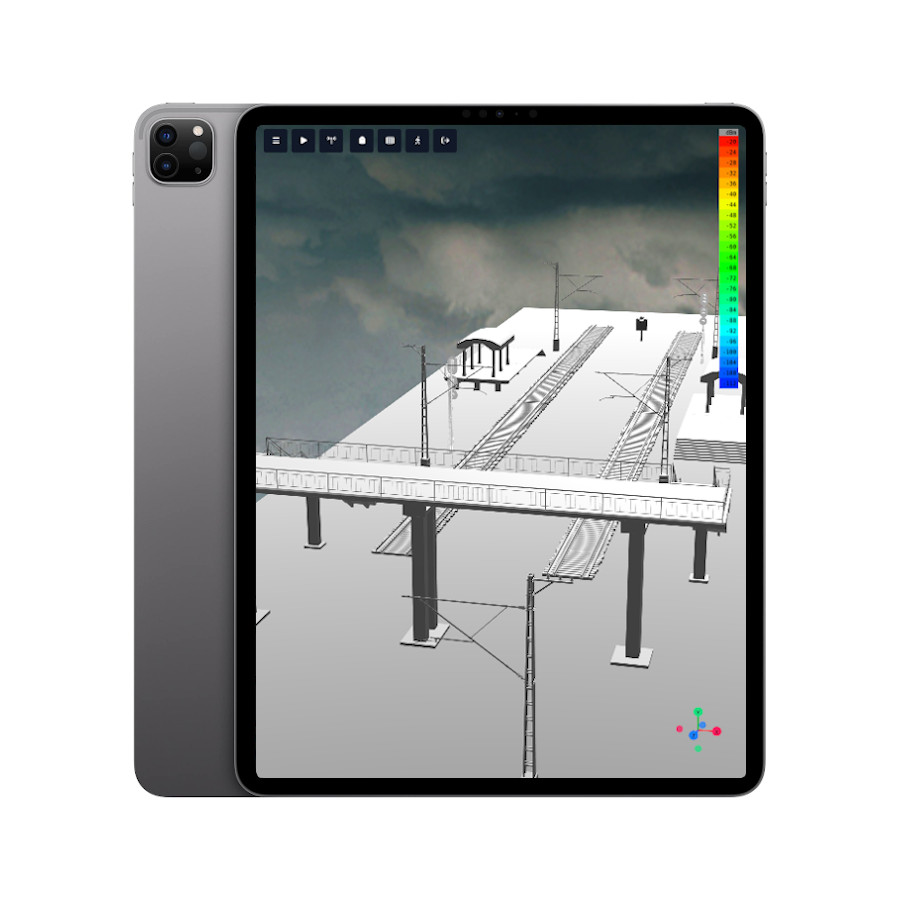
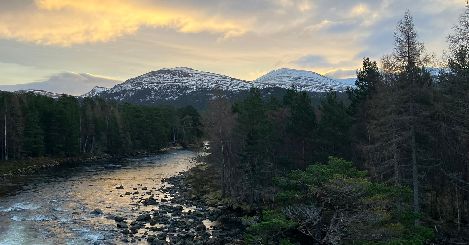
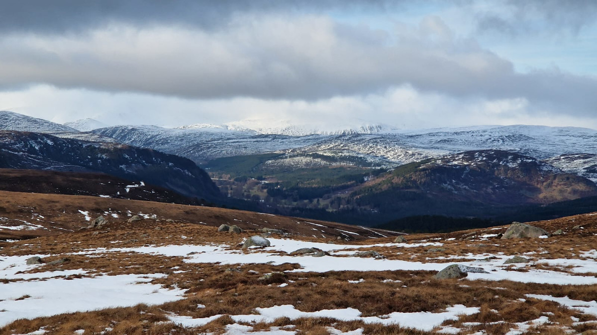
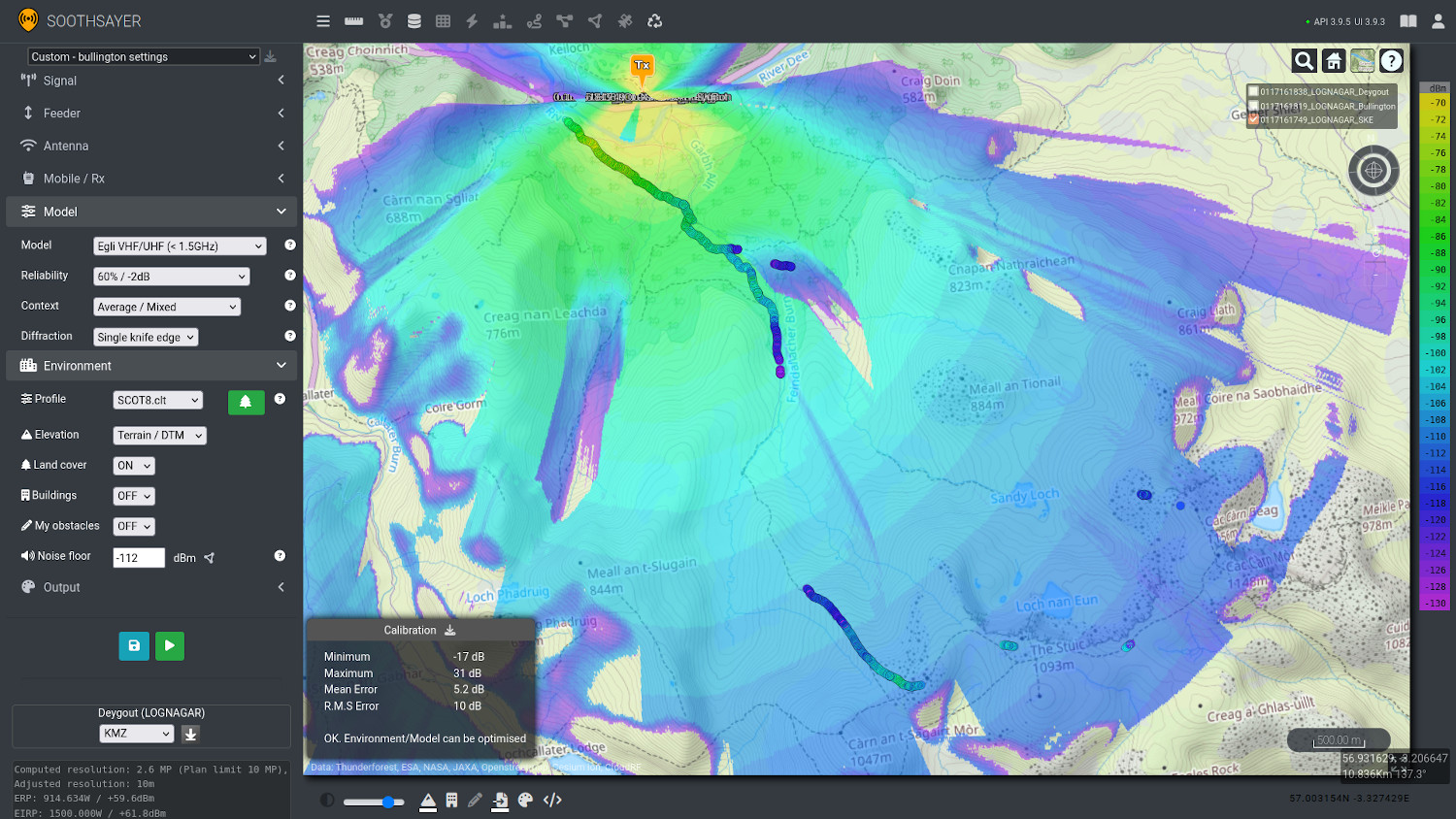
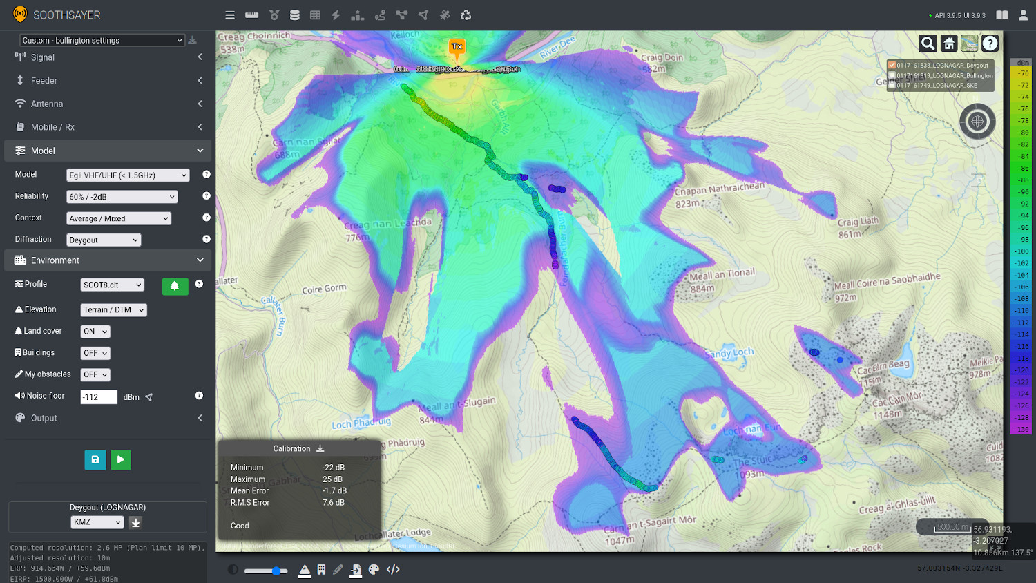
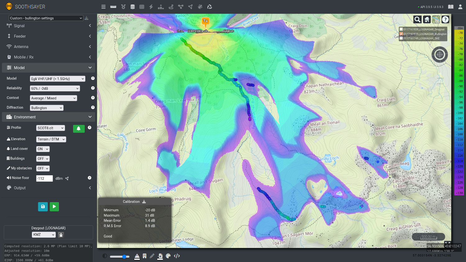
Snow covered trees

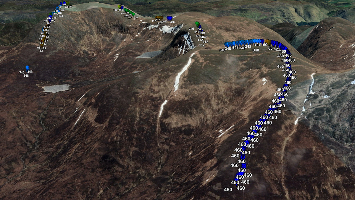
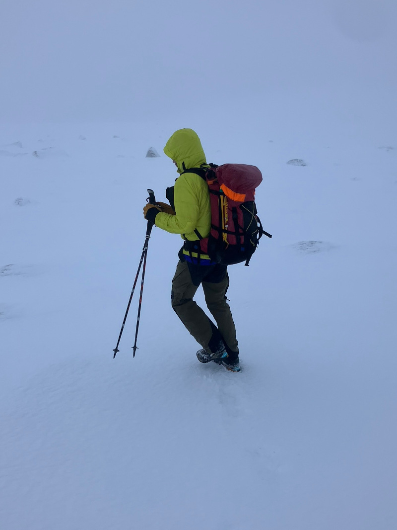
Taking the test up a gear to the Arctic circle, we collected LTE survey data using the RantCell survey app from the top of Finland across multiple bands to investigate the accuracy impact of thick snow on trees.

Snow is a lattice of water which reflects and attenuates RF so is challenging to simulate, especially as it changes!

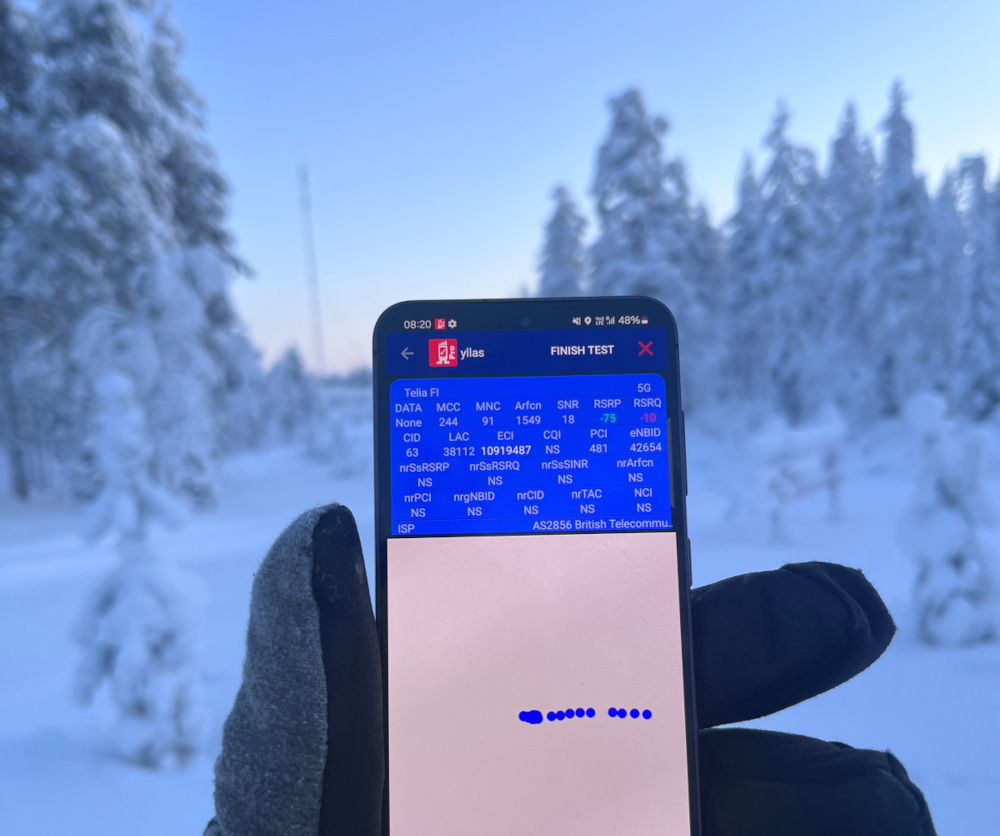
The field data collected gives us RSRP (Reference Signal Received Power) from two LTE bands (band 1 and band 3) from our tower of interest. This gives us a good opportunity to use one data set to calibrate a model and then use the second set to see if model prediction performance remains consistent across frequency. The frequencies of the two bands do make model selection more limited as band 1 (~2.1GHz) sits above the threshold for Okumura-Hata, its extension COST-231 and Ericsson 9999.

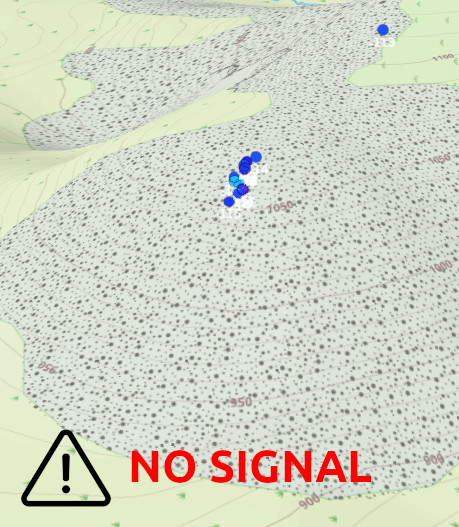
For the data itself we are looking at a small section of coverage near the tower surrounded by large snow-covered trees in undulating terrain. The collection was performed on a ski track under the trees which was often covered by a tree canopy.

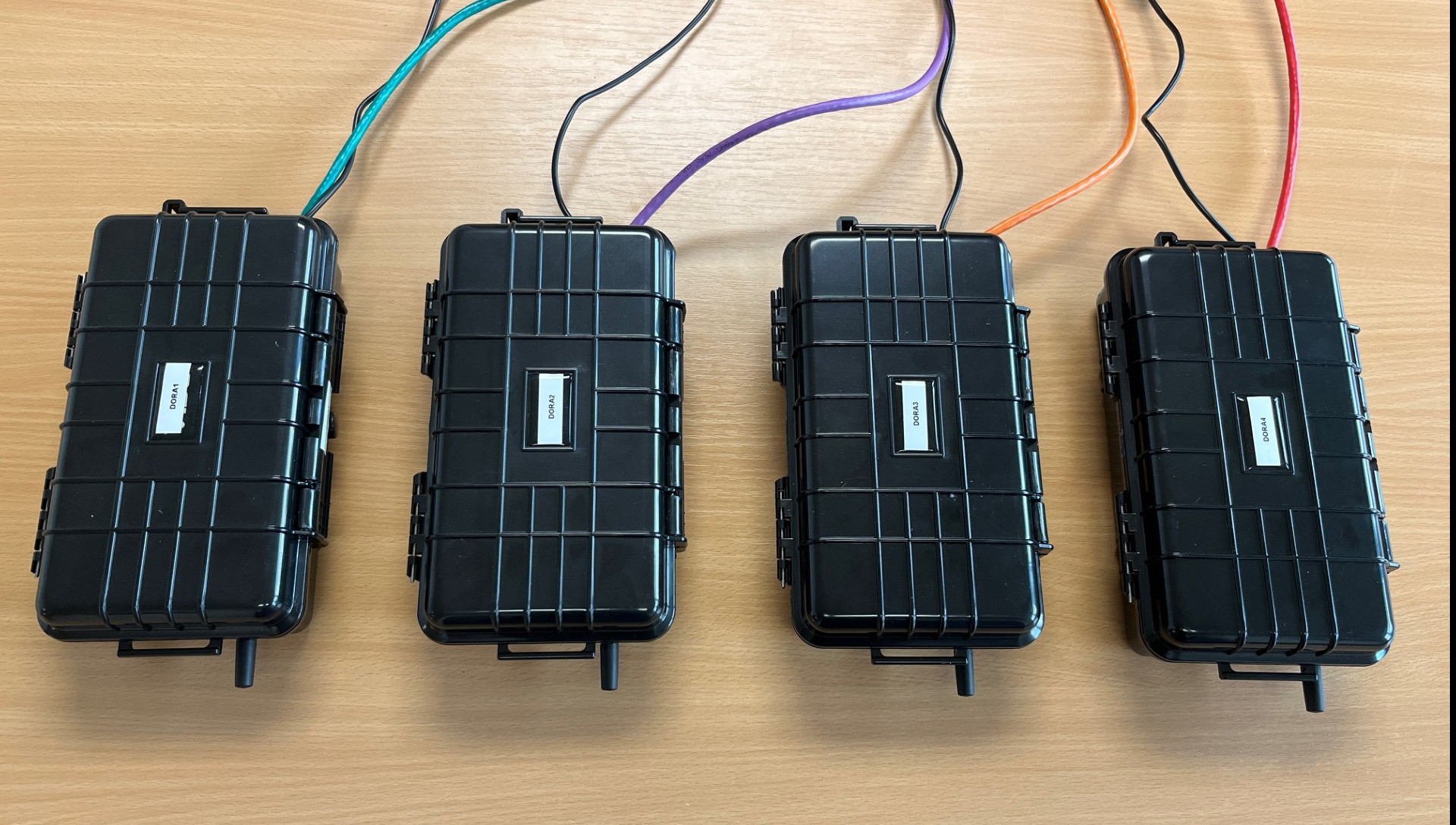
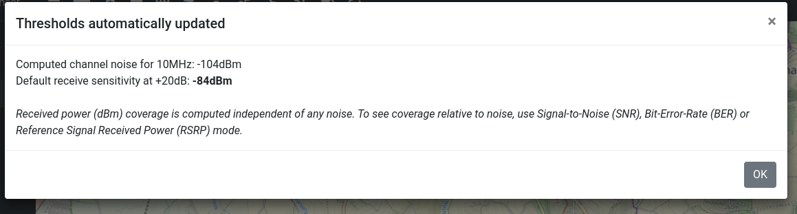
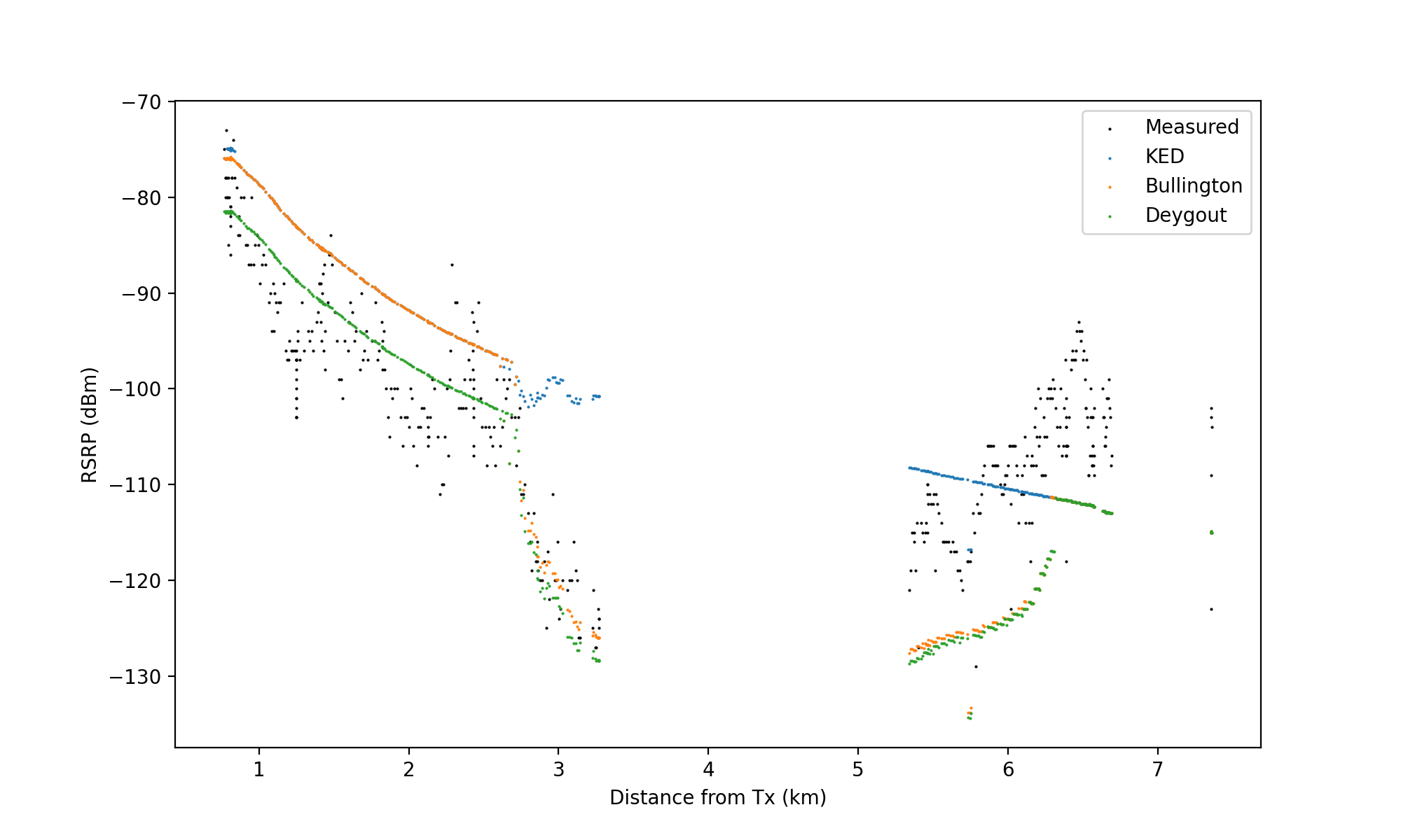
The signal RSSI was calculated as 30dB above measured RSRP using the known 20MHz bandwidth and the data fed into our calibration tool to plot the points. From the app’s data, we know the LTE bands for each of our data sets, so we have a centre frequency and bandwidth. Using the photograph of the mast we can approximate its height at 60m. With the mast location set, we can then make two sets of predictions for both 1820 MHz and 2140 MHz down links and compare model performance across both. We will use P.525 as our free space reference model.

1820 MHz

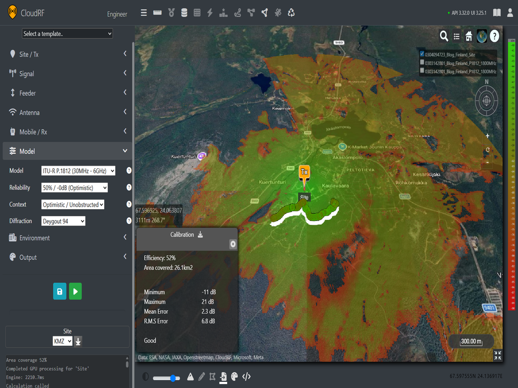
• ITU-R P.1812 (Mean: 2.3 dB, RMS: 6.8 dB)
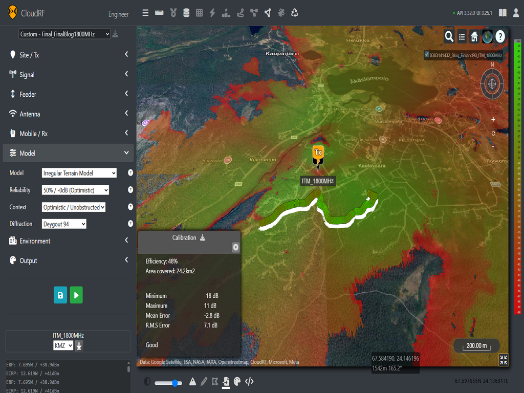
• Irregular Terrain Model (Mean: -2.8 dB, RMS: 7.1 dB)
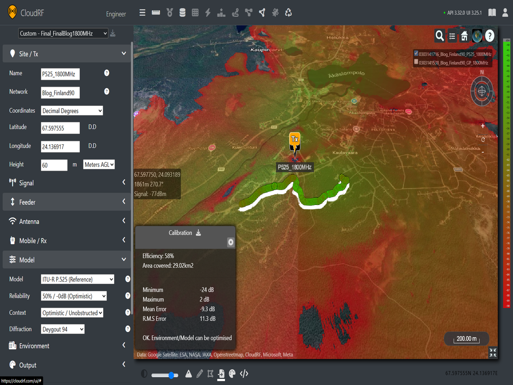
• ITU-R P.525 (Mean: -9.3 dB, RMS: 11.3 dB)
• Ericsson 9999 (Mean: -8 dB, RMS: 10.5 dB)
• General Purpose (Mean: -23.3 dB, RMS: 24.2 dB)
• COST-231 (Mean: -43.9 dB, RMS: 48 dB)

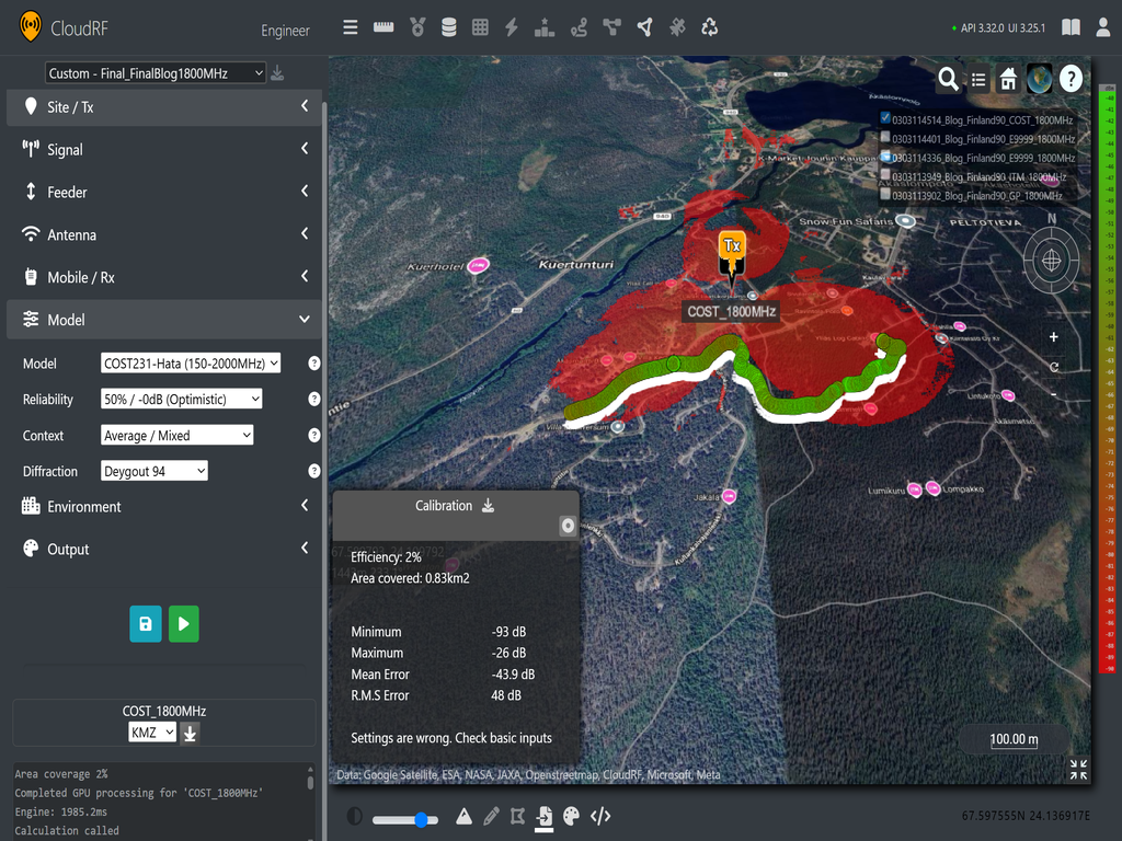
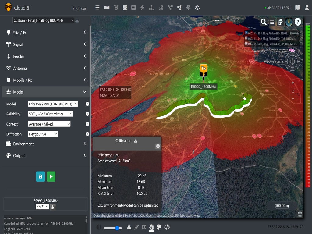
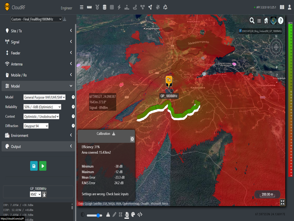
When comparing the predictions to the 1820 MHz data sets, we can see that P.1812 and ITM are close predictors of the measured values. Additionally, when Ericsson 9999 is used with an average/suburban context, it gives an okay estimate, but has a much smaller coverage area overall, suggesting that more tuning is required to better match the attenuation caused by the large snow-covered trees. General Purpose is over attenuated which was not surprising given our free space path loss is a close fit and the 20 dB offset was added following tests with ground based tactical radio networks, not 60m masts. COST-231 is unusable which was expected given it is well outside it’s intended environment.

To test consistency, we can now look at the test results at 2140 MHz. Unfortunately, we can’t include Ericsson 9999 or COST-231 as the operating frequency is too high. However, we can test the Stanford University Interim (SUI) model which is rated for above 1.9 GHz.

2140 MHz

• ITU-R P.1812 (Mean: -5 dB, RMS: 9.2 dB)
• Irregular Terrain Model (Mean: -5.1 dB, RMS: 9.6 dB)
• ITU-R P.525 (Mean: -9.4 dB, RMS: 12 dB)
• General Purpose (Mean: -23.4 dB, RMS: 24.6 dB)
• SUI (Mean: -69.3 dB, RMS: 72.9 dB)

From this comparison, we can again see similar results. ITU-R P.1812 is again providing the best prediction, followed closely by ITM. The observation for P.525 and General Purpose remains the same. The SUI model is heavily over attenuating using an unobstructed context. This is not surprising when looking at the generic path loss graphs shown previously shown. SUI has consistently been the most conservative microwave model in our collection and based on the performance in comparison with other models it will be retired from our API in due course.

LTE conclusion

Looking at the two set of predictions, we can see consistency in performance from both P.1812 and ITM with P.1812 giving the best fit. Their coverage maps are generally consistent shapes with themselves and each other and we see more attenuation through the trees at our higher frequency as expected.

Our two models are showing their utility by giving accurate predictions despite heavy snow based on terrain and clutter data alone. The next question for these two models now is how to tune the clutter for each frequency for a better match.

Key findings for choosing a Propagation Model

Having conducted tests across six locations with different datasets and frequencies, we’ve gained insights into how each propagation model performs. The results of those tests have been broadly consistent with deterministic models like ITU-R P.1812 and its legacy predecessor ITM being consistently accurate before calibration and clutter tuning.

The old empirical models can be accurate, but they require the correct context to make an accurate prediction and without test data, it is difficult to tune them to their respective environment due to their fixed path loss curves. This is why we are recommending ITU-R P.1812 as our default model for VHF, LoRa and LTE propagation when using Cloud RF. You can still use Empirical models, but you’ll have to commit to collecting field data for tuning.

To further improve accuracy, users can tune our clutter profiles with variables such as tree heights or average attenuation through buildings. To understand where these values come from, please check out our past model and clutter improvements blogs or if you want to accelerate the process, see our calibration with machine learning demo with sample code on our Github.

What about Machine Learning?

The promise of Machine Learning models to improve accuracy (and speed) is tempting but it depends upon an enormous quantity of accurate training data. In our experience, ML researchers struggle to generate the vast quantity of accurate and expensive test data needed to develop even small demos.

Given enough training data, an ML model could be quicker and just as accurate as physics based simulation or potentially a drive survey.

However, it is naive to criticise the performance of physics based simulation in favour of ML as the model generation relies upon the former to train the model which creates a dichotomy whereby ML developers need to both criticise, and rely upon, simulation tools to develop an accurate model (and secure funding). There is a solution to this which requires academic honesty and a mature and scalable API but one of those requirements is harder to come by than the other.

Further Reading

Fast simulation calibration with Machine Learning

Model and clutter improvements

SG 3 Databanks – ITU

CloudRF model menu

Background

Radio Direction Finding (DF) is the art of determining the location of an emitter and is used in search and rescue, coastal surveillance, law enforcement and defence. There are different techniques using power and phase but the output for a single sensor is normally a Line of Bearing (LoB) which points towards the emitter.

If you’ve ever seen DF depicted in marketing or an info-graphic, you’ve likely seen three geometrically distributed sensors surrounding an emitter which produce a high accuracy position fix (PF) where their lines of bearing converge.

In the real world, DF systems are expensive and require specialist training so are in short supply. It is far more common for these systems to be used in isolation so operators must determine an emitter’s location with a single LoB and a map study. For powerful signals, the search area could be vast.

Guessing the signal power

For a signal to be tasked for DF, it’s frequency is already known. With signal classifiers increasingly integrated into receivers, and now even open source, the signal type may well be known which helps answer a key question: what is the signal’s transmit power?

When a new signal is detected, it could be in the room next door or in the next county. Knowing the signal type and ideally the hardware is key to estimating the distance, as you can lookup the possible power levels from a data sheet.

A portable radio has variable power levels: For a DMR radio with low and high power at 0.1W and 4W these can be put into a basic path loss model to determine the possible distance. Using the Friis reference model with a detected signal of -80dBm for example, a 1GHz signal could be 2.4km or 15km away in free space.

This significant variation with the possible distance is where modelling can add value to reduce the vast search area.

For the example radio, these power values in Watts must be converted to decibel milliwatts (dBm) for consistency with the path loss modelling and to establish the range in decibels which will inform simulation parameters. In this case, low power is 20dBm (0.1W) and high power is 36dBm (4W) for 16dB of uncertainty.

In an obstructed environment such as a forest, this uncertainty represents a shorter distance than in free space where again, modelling can add value. A counter drone system is an example of a free space problem.

Link reciprocity

A radio link is not symmetrical due to how and where obstacles impact the fresnel zone which is the cone of power an element radiates. Even if you have line of sight (LOS) between two even power stations, you can still get different received power levels from A to B than B to A.

This matters as we cannot model the emitter since we don’t know where it is! We can only model the receiver location.

In our experience, the difference is measured in single digits and is small compared with noise which will make a bigger impact on a link’s viability. If you are operating at the edge of a system’s link budget then the reciprocal difference may be enough to make a link one way only.

For modelling a receiver we need uplink (talk-in) measurements instead of downlink (talk-out) which we normally collect for clutter and model calibration.

Field testing

We conducted several field tests to integrate our API using a budget commercial DF receiver, the KrakenSDR. This compact entry level unit gave us a LoB (with 8 degrees of error) we could work with but as it used 8-bit SDRs, we could not rely upon the received power level as low resolution SDRs can not represent weak signals.

After a false start with a 12-bit SDR designed for the amateur community and interfaced with SoapySDR, we used a professional RFEye receiver which aside from having superior measurement accuracy and sensitivity is a turnkey solution with a web API which we have integrated with our API previously.

Test system

Our test system grew in scope from a Kraken with a Pi to a network in a box with a bespoke management and signal logging interface. Key to this innovation was not creating a budget DF system which we needed to collect data but the employment of an edge modelling capability on a Raspberry Pi 5.

Our goal was to develop a hardware agnostic script which our customers could use to enhance their DF data.

Hardware

• The Line of Bearing came from a KrakenSDR with a circular 5 element array upon a 2m telescopic mast.
• The processor was a Raspberry Pi5 running our test software and SOOTHSAYER v1.10
• The radio traffic was generated by a Tait DMR portable radio equipped with a programming cable connected to a Pi4.
• The power measurements came from a CRFS RFEye connected to an elevated monopole antenna.
• A pair of sensecap meshtastic LoRa trackers were used for GPS tracking.
• A laptop and tablet running ATAK were used to manage the system and observe the output as a KML.

Software

To automate data collection, we developed test software to collect data from the SDR and DF receiver simultaneously and model them using our API. The DMR radio was configured to broadcast telemetry periodically which provided a regular target signal and the out-of-band meshtastic tracker provided a precise location within the trees.

We couldn’t use a second DMR radio to receive the telemetry as bi-directional radio traffic risked spoiling the data.

The modelling came from SOOTHSAYER 1.10 which was installed upon the Raspberry Pi 5. This also provided the map tiles for a web based logging system which displayed live signal readings. Only one (CPU) API call was necessary per test cycle to generate a grey scale Path Loss map in decibels (dB) from which subsequent received power heat maps in decibel milliwatts (dBm) could be rapidly derived using a simple formula.

The path loss simulation needs refreshing if either the location, frequency or height change but is power agnostic. The client script queries this path loss map using known (or assumed) radio power levels.

Results are presented as a network KML which can be consumed on standards based geo-viewers like ATAK.

Challenges

We took our ‘Temu DF system’ out twice but we couldn’t collect as much data as we wanted in the time available due to different constraints such as the weather or just running a small business.

A decision to avoid vehicles and buildings was made to avoid reflections which meant we had to run the equipment from travel batteries. The power budget for the Pi5 (30W), KrakenSDR (12W) and RFEye (5W) was 47W which was more than we normally test with so it reduced our endurance.

We encountered local radio traffic on our licensed channels due to the choice of locations overlooking the city. This was easy to discount at the start of the test when our signal was obvious but became a nuisance as it faded into the trees and ultimately tainted our test data since we were triggering on power.

Old data to the rescue

After several frustrating tests where a lot of time was spent climbing local hills, calibrating DF and chasing false positives, we elected to reuse a rich data set from an antenna field test last year which included bi-directional links for a UHF radio on a moving vehicle.

This data was attractive as it included the uplink and a good variety of obstacles including houses, trees and hills as well as LOS links which are all useful for calibration. Before we could conduct DF analysis with the uplink, we calibrated the local clutter using the downlink, as we do routinely for calibration. This is a standard process we have developed a feature for in the web interface as well as a supporting video tutorial. Using our new 2m tree height data, we were able to improve upon last year’s score.

As we did not collect lines of bearings during that model test, we had to simulate these using the known vehicle location for which we used 10 degrees of azimuth error.

Analysis technique

To compute the effectiveness of this technique we calculated the area of the 10 degree arc where the vehicle could have been, with a radius of 6km representing the maximum range in this test.

This gave us a search area for a given LoB of 3,141,593 m2.

Our analysis script calculated a high resolution grey scale heatmap using SOOTHSAYER’s API which was referenced with collected power readings. To compare path loss (dB) with received power (dBm) we used the known radio power of 2W (33dBm) within a link budget formula to generate received power which was compared with measurements.

RSSI (dBm) = Radio Power (dBm) + Gain (dBi) - Path Loss (dB) - Losses (dB) + Receiver Gain (dBi) - Receiver Loss (dB)

Where the difference between measurements and simulation was within tolerances of our colour key, we styled that pixel, otherwise we eliminate it from the search area and set it to transparent.

The result is an accuracy heatmap defined by a traffic light colour key. The levels we chose for our “known power” assessment were 1, 2 and 3dB. By showing 3dB of error we allow for receiver error and reduce the risk of false negatives where a matching location might be discounted.

When the radio power is known, we can produce more accurate results.

When the radio power is unknown and the hardware/signal is known, we can simulate the minimum and maximum power to generate a dynamic range for the analysis. We used a low power value of 20dBm (0.1W) and a high power value of 36dBm (4W) for a possible power range of 16dB so our “low accuracy” colour key was 14/15/16dB.

We repeated the analysis with known and unknown power levels to compare accuracy.

Results

Analysis of data revealed the simulation heatmap significantly reduced the search area. As expected, knowing the radio power helps greatly but even with unknown power the search area was reduced to 32% of what it could have been for a conventional 6km arc.

Even when radio power is unknown, the search area is reduced significantly

	Known Power (2W)	Unknown Power (0.1 or 4W)
Best case	0.01	0.03
Worst case	27.33	64.37
Average area	7.93%	31.51%

The amount of benefit was relative to the terrain and clutter: For example, where there were no obstacles or a single consistent obstacle such as a forest, the result was a focused band of probability without any false positives.

Where there were multiple obstacles such as a hill and a forest, false positives appeared which depending upon the ground could be discounted by an observer. This was to be expected given the pixel picking which is taking place.

A tight traffic light schema, with tuned clutter, was better than a loose schema with larger error margins. The reason being that it will show much less false positives.

Video and KMZ

This video is a sped-up compilation of time stamped KMZ layers viewed on Google Earth showing the vehicle’s route around the sensor. Where the vehicle disappears, no signal was detected.

The KMZ is available here and works best in Google Earth.

Conclusion

This testing proved that the effectiveness of a single LoB can be improved greatly with modelling but the concept is only an improvement if the analysis is automated as doing this manually would not be faster than a map study.

The reason this analysis isn’t performed regularly by DF systems today isn’t for a lack of LoBs and RSSI measurements but rather a lack of APIs with which to exploit this information. Current RF planning software exists as a user interface which requires manual, and skilled, operation. Furthermore, the capability often exists in the wrong location on a high performance desktop computer, disconnected from edge sensors.

By putting this API at the edge on small board computers (SBCs) such as the Raspberry Pi 5 or Nvidia Jetson, a DF system’s effectiveness can be improved. Through open GIS standards like KML, the result can be consumed on open standard GIS systems like ATAK requiring minimal integration effort to add a powerful capability.

Looking forward, we are speaking with open minded vendors about adding this API to enhance existing systems.

If you’d like to improve your LoBs, get in touch with us or one of our regional resellers.

Links

SOOTHSAYER server: https://cloudrf.com/soothsayer

Kraken SDR: https://www.krakenrf.com/

DF integration demo: https://github.com/Cloud-RF/CloudRF-API-clients/tree/master/integrations/DF

API schema: https://cloudrf.com/documentation/developer

We’ve published a series of video tutorials for HF novices to bring to life HF theory around the topics of Frequency selection, Antenna fundamentals and forecasting.

HF communications is very different to terrestrial communications and given the right frequency, time of day, and antenna, you can achieve long range links in excess of 1000km with only a few watts of power on a HF Dipole.

CloudRF’s API uses the proven VOACAP engine to create accurate HF predictions considering a number of factors. Using this tool, you can plan long range resilient links and anticipate the (time based) surprises HF throws up…

Frequency Selection

Time is critical to HF communications. As sunlight changes throughout the day, so does the range of usable frequencies. A common strategy for round the clock communications is to maintain a day and night frequency. These can be identified using the VOACAP powered path tool in CloudRF.

This tool reports the Signal-to-Noise ratio against time for different HF frequencies.

Antenna Basics

Once a frequency has been identified, an antenna must be constructed to the right dimensions.

The antenna of choice for many long range HF links is the half wave dipole. This simple and efficient design uses two fixed length elements and a center feeder to bounce signals off the ionosphere.

To get the wavelength for your frequency divide 300 by the frequency in MHz.

Height

The height of the antenna will change its radiation pattern and the take off angle.

Achieving at least a quarter wavelength is recommended for efficiency (and practicality) as the long HF wavelengths make a half wavelength too high for most masts. For an 11MHz signal, the height would need to be 6.8m for example.

Azimuth

HF patterns are directional and must be orientated towards a distant station. For some antennas, like long end fed wires this is as simple as pointing the wire towards the station.

For a half wave dipole, which has a donut shaped radiation pattern, it must be broadside towards the station as it has nulls where the wire ends are. A bad azimuth can be forgiven at short range but will determine the potential range.

Feeder loss

Using a feeder co-axial cable will reduce the efficiency of your system. The effect increases with length so you should aim for the shortest, low loss, feeder possible. The impact of the feeder can be simulated even if you don’t know the cable type by entering 1 or 2dB into the feeder loss option.

Forecasting

Sunspot R12

The Sunspot index number describes solar activity which follows a 10 year cycle. When the number is high, there is increased solar activity and better refraction. The different between a good and bad year within the cycle is around 6dB which on the S Meter scale is equivalent to two levels, or the difference between success and failure.

This can be predicted and the random element budgeted for using the model’s reliability value.

Simulating indoor radio coverage for first responders has been made simpler thanks to a new capability called Phase Tracing.

The novel design was influenced by the 2017 Grenfell Tower inferno, where radio communication in concrete stairwells was highlighted as a major problem. The Grenfell inquiry highlighted radio and training issues in the report, which had a section dedicated to communications.

During the inquiry, expert witnesses were unable to demonstrate how far a signal would travel within the tower, even with the availability of indoor planning tools. Estimated distances offered to the inquiry were based upon empirical measurements from elsewhere and were at odds with witness statements from firefighters who reported losing communication after only four floors and communicating with paper notes.

The intensive computation required to perform a true 3D simulation with reflections has been made practical through developments in graphics processing. As a result, accurate radio coverage in stairs, tunnels and elevator shafts can be simulated, at the network edge, by an operator with minimal training.

In contrast to legacy indoor planning tools, which use floor plans and images; Phase Tracing is designed for critical communications and industrial markets in challenging and dynamic 3D environments, represented by digital models.

Models not floor plans

Phase Tracing represents a leap forward for radio simulation from overlaying images upon a 2D map or floor plan, suitable for an estate agent, to using a digital twin 3D model which considers all floors, and the obstructions in between from stairs, to air ducts and pylons. Simulating reflections is critical for indoor modelling which is a pillar of the design.

There also exists a huge gap in the market between indoor simulation packages and the skill required to use them effectively, and first responders who are left guessing where they will lose communications on a stairwell. This gap has been closed by developments in computation, namely GPU processors, and web technologies which mean this powerful API can be used from a low power touchscreen device.

A little movement…

For RF theory students who are taught the impact of multi-path; they now have a tool to visualise and explore this important concept; so they can see why “a little movement may cure a dead spot”. Better still, they can identify constructive “good” multipath they didn’t know about.

The GPU accelerated engine reads and writes to open standard glTF models and uses ray tracing techniques from computer games to bounce photons around the model. With the addition of phase, multi-path artefacts such as signal “dead spots”, where out of phase signals on the same wavelength cancel each out, can be modelled.

The number of reflections, material attenuation and scattering properties can be configured. This is essential for modern buildings which are built with materials which disrupt radio communication.

Applications

Phase Tracing has a distinct advantage over 2D modelling for the following 3D obstacles in most wireless industries.

• Stairs
• Tunnels
• Bridges
• Towers
• Pylons

Design

The Phase Tracing capability is built upon our 3D API which we launched last year with a blender plugin. The API can be called directly to integrate the output into other model based systems, or even viewed in a standalone HTML5 viewer.

The interface and API is radically different to our map based Globe. For starters there are no Geographic coordinates, positions are in Cartesian XYZ co-ordinates relative to position 0,0,0. This is so you can work with models which might not have a geo reference or in the case of design, might not even exist yet.

Photons and Phase

The 3D engine is a CUDA accelerated pipeline, like our 2D GPU engine, which processes jobs asynchronously to service multiple users. It creates a voxel model from a glTF file which it then radiates photons around. A photon will reflect from obstacles until it runs out of energy or reaches a reflection limit. Unlike Ray Tracing, a legacy technique for indoor modelling, these photons maintain their phase so multi-path can be simulated in all directions.

Each reflection costs several decibels of power typically so there is a practical limit, depending on the material, after which it will be too weak to be useful and the photon should be killed. The engine can model up to 30 reflections per photon which do not impact performance so much as the number of photons, currently set to 2^e6. The required number of photons depends upon the model: If you have a small office and need to decide where best to put a Wi-Fi Access Point you don’t need many.

If however, you need to model reflections up a stairwell, along a corridor and into a flat you need millions. This isn’t fast, or pretty, but such is the nature of critical communications. We’ve fixed the photon limit on CloudRF to deliver a calculation in under 30 seconds for a large model. A small model will be quicker.

VR/AR support

The cross platform interface uses three.js and the WebXR library which supports Virtual Reality and Extended Reality devices. We have a XR branch we’re playing with on a Meta Quest but are having a headache issue as it is so immersive you get vertigo exploring tall models. Once this is sorted, likely by AR, we’ll merge it. Last year the 3D output was integrated into a third party Hologram interface.

Demo Gallery

We have an interactive demo gallery of 3D models you can explore on our Github pages. To use these demos you will need a WebGL capable web browser like Chrome. You can use your mouse to zoom in and explore the models or download them as GLB to view on your phone using an app like glTF viewer. iPhones support these GLB models natively.

Roadmap

The API and version 1.0 of the interface have been published. The API can be used by Silver and Gold customers and the interface is restricted to Gold only presently whilst we build more infrastructure to support this.

June 2024 – 3D API

• Upload glTF model
• Perform multi-site simulation using transmitter parameters
• Configurable material attenuation
• Configurable reflections and attenuation
• Blender plugin
• 1e6 photons
• Mega voxel limits

Jan 2025: Phase Tracing 1.0

• Cross platform web interface
• GLB Model management (Add, Remove)
• Local model caching
• 3D antenna models built from user’s antennas
• Click to aim
• Configurable reflections, resolution and default material density
• 2e6 photons
• Save/Load settings as JSON

TBC: Phase Tracing 1.1

• Official VR/XR support
• GLB download
• Material manager for construction materials
• Biasing for speed boost
• Configurable photon limits – linked to plan

Sample GLB models

Upload these glTF binary models into the interface or another tool such as this handy free viewer.

You can validate your models with another free tool here.

Our latest field test was focused on drive testing novel antennas by UK SME Far Field Exploits (FFX) around the Somerset countryside with Trellisware radios.

Previously, we validated diffraction models using LTE800 in the Mountains. The outcome of that cold test highlighted Deygout as the most accurate diffraction model when paired with empirical cellular models. For this much warmer antenna drive testing, we used lower frequencies and a lower mast in an area with many trees which presented a challenge for both legacy cellular models and LiDAR.

Testing highlights

• Average Root Mean Square Error of 7.4dB
• Average Modelling Error of 4.4dB
• Automated data collection with ATAK plugin
• New “General Purpose” model developed
• New “GP” clutter profile for use with GP model

Test setup

The test area was in and around the small town of Somerton in Somerset. This town sits in rolling countryside featuring farms, high hedgerows and blocks of trees. A railway line with road humpback bridges bisects the town. The town has a small housing estate under construction which did not feature in our buildings data.

The base station was a wide-band Omega panel elevated 5m above the ground and connected to a Trellisware spirit radio. The radio was operated across several UHF bands, each with 1.2MHz bandwidth, and live positions observed on WinTAK using cursor on target (CoT).

The antenna testing vehicle was fitted with a roof mounted magnetic antenna bracket which connected to a spirit radio. This mount allowed different antennas to be swapped out. As a result we were able to test both a Hascall Denke MPDP675X4 and a FFX Sigma 3.

Data logging

We know customers and OEMs like to voice opinions about radios, waveforms and antennas but without solid measurement data it’s just noise with a lot of bias and emotion.

Data beats emotions every day!

As an antenna OEM, FFX developed the ATAK spectrum survey app to streamline collection of field measurements for antenna testing in different environments.

The logging application used the Trellisware radio’s API to fetch link metadata from the local radio and save it to the SD card as a CSV file.

The ATAK plugin enabled a large quantity of high quality measurements to be efficiently collected. As a result we were able to execute several test cycles in a short space of time – just as well as it was hot (for the UK) and Harry had no air conditioning…

The CSV files were downloaded from the phone and loaded into the CloudRF calibration utility for analysis.

The survey data was filtered to remove results weaker than the theoretical noise floor at -113dBm.

We were planning to use a measurement error of 2dB for the high quality radios (a cell phone is 3dB) but owing to the high temperate of the mobile radio in the car we used 3dB as receiver performance degrades with temperature.

At first look

The first pass comparison of the data showed a ~15dB delta between modelling and field measurements with LiDAR, prior to tuning. Using the ITM model and a high reliability value (99%) this only reduced several decibels and clearly needed more work. Ideally the model should align within 10dB so clutter tuning can then be used to reduce this towards 6dB.

ITM uses the complex Vogler multi knife edge diffraction model which is accurate for hills but needs tuned clutter to handle soft obstacles. Using cellular models, as we did in LTE800 field tests, didn’t produce the same results due presumably to the lower mast height and frequencies, even when enhanced with Deygout diffraction.

A new model

Through curve fitting we identified alignment with the P.525 reference model and a 20dB constant representing observed system losses. When enhanced with the Deygout 94 diffraction model this produced excellent alignment with the more challenging beyond-line-of-sight areas. Many signal paths on the route had multiple obstructions so a multiple knife edge model (MKED) was essential.

We have created a new model from these settings called the General Purpose Model. It is frequency and height agnostic which makes it ideal for ground and air based links and much more versatile than empirical equivalents which must be operated within a restricted performance envelope. Like all our models it must be used in conjunction with a diffraction model and tuned clutter to deliver accurate beyond line of sight results.

In our opinion, modern developments in processing and clutter data especially have rendered legacy empirical models largely obsolete. The modern way to fit modelling to measurements is to focus on precise clutter data not old path loss curves.

In the screenshot below, the car drove up a hill where it fell off the network behind a prominent knoll before reacquiring the network later on. This knoll was the second of two obstructing hills for this section of the route. The modelling predicted more coverage due to the chosen receive threshold, -107dBm, which was based upon 6dB above the thermal noise floor which was -113dBm at 1.2MHz bandwidth. It is very likely local noise was slightly higher.

ITU clutter values

Without clutter, the General Purpose (GP) model will be optimistic in most ground environments. It will be accurate over bare earth but where obstacles are present, it needs land cover and a clutter profile. Prior to developing the GP model, we did most of the tuning in the model using reliability (%) and only fine tuned with the clutter.

This is why older CloudRF clutter profiles eg. Minimal.clt have low values such as 0.05 dB/m for trees. With the GP model, the model itself is very simple and most alignment takes place within the clutter (profile). As a result, the clutter values used for GP are much denser. Our GP profile, created for this test has trees with a density of ~0.5dB/m, aligning with ITU-R P.833, attenuation in vegetation.

Diffraction logic has been re-balanced to accommodate ITU clutter values. Users using either the default ITM model or models without land cover are not affected. Legacy clutter profiles such as Minimal have not changed but you are advised to try the new GP model and associated GP clutter and see the difference for yourself.

Test parameters

Bandwidth: 1.2Mhz

Feeder loss: 1dB

Receiver height: 1.5m

Receive sensitivity: -107dB (6db above noise)

Noise floor: -113 dB

Model: General purpose / ITM

Reliability: 60% / 90%

Context: Average

Diffraction: Deygout 94 / Vogler (ITM)

Clutter Profile: Buildings 3dB/m, Trees 10m @ 0.5dB/m

Radius: 6km

Resolution: 5m

Results

The following table of results were from measurements conducted with the same base station, vehicle and radios. Only the vehicle antenna, and frequency, were changed in between tests. Once calibration had been achieved the area covered was extracted from the modelling. This is typically inverse to the frequency so a low frequency has better coverage than a high frequency at the expense of bandwidth – and both matter.

There are two standout results from the data: First is the low RMSE accuracy for the new GP model with tuned clutter compared with LiDAR which is satisfying given the challenging terrain and the second is the performance of the Sigma 3 on a frequency it is not officially rated for as it has a bottom end of 350MHz. The best alignment with the same settings was found to be with -5dBi receive gain confirming the antenna can be operated lower, and at range.

Once again, DTM with clutter has proven to be superior to LiDAR.

Antenna test	Model + Diffraction	Clutter profile	DEM	Receive gain dBi	RMSE error	Modelling error	Modelling area covered km2	Modelling area covered %
Hascall Denke MPDP675X4 on 1.4GHz	GP (60%) + Deygout 94	GP	DTM + 10m Land cover + 2m Buildings	2	9.4	6.4	19.2	17
Hascall Denke MPDP675X4 on 1.4GHz	ITM (90%)	N/A	LiDAR	2	15.2	12.2	12.4	11
FFX Sigma 3 on 415MHz	GP + Deygout 94	GP	DTM + 10m Land cover + 2m Buildings	2	6.6	3.6	89.9	79
FFX Sigma 3 on 415MHz	ITM (90%)	N/A	LiDAR	2	18	15	72.7	64
FFX Sigma 3 on 287MHz	GP + Deygout 94	GP	DTM + 10m Land cover + 2m Buildings	-5	6.2	3.2	86.1	76
FFX Sigma 3 on 287MHz	ITM (90%)	N/A	LiDAR	-5	15.1	12.1	63	56

The scatter plot for the 1.4GHz data shows the simple GP model to align closer to field measurements than the much more complex ITM model. Our conclusion is that the ITM model, and it’s Vogler diffraction, developed in the 1960s, pre-dates developments in computing and precision clutter so provides good performance across multiple hills, at range, but is inadequate for macro planning at “street level” resolution where density of obstacles must be budgeted for.

ITM continues to be a solid UHF broadcasting model but it was designed for hard obstacles. Retro fitting it with soft clutter, as we have done can improve its performance several decibels but for maximum accuracy, the simple General Purpose model with tuned clutter provides superior results.

Results Gallery

Tuned coverage and survey data is displayed on the same map showing the RMSE and Mean error.

Look ahead

The General Purpose model will go live on CloudRF in early July 2024 following more testing and then into SOOTHSAYER 1.8 later in the year.

The problem with tunnels and stairs

Whenever there’s been a major incident involving emergency services in complex urban environments the inquiry report has consistently highlighted radio communications failure despite significant developments in radio communications and 3D technology since the infamous 1988 Kings Cross Fire on the London Underground. The following tragic incidents all featured tunnels, stairs and communications failure:

• The 1988 Kings Cross Fire report highlighted radio communications only worked when they were in line of sight.
• The 2007 London underground bombings report highlighted that radio communications from trains to network control were inadequate or non-existent.
• The 2017 Grenfell tower fire inquiry highlighted inadequate radio communications between the incident control on the ground floor and fire fighters higher up the tower.

Limitations of (2D) radio planning tools

Radio planning tools are not used in emergencies. They’re complicated, slow and require a lot of knowledge to produce an accurate output. Even if a skilled operator were able to model a site before the event, currently they would be expected to model each floor of a multi-story building in isolation due to the “floorplan” design of current software.

The problem is indoor planning tools are built for corporate clients to achieve seamless Wi-Fi in every corner of the office, not to help a fire chief deploy a mesh radio network down stairs and then along a tunnel. The top end tools can do limited multipath, slowly, but not as an API which can be consumed by a third party viewer…

Most radio planning tools on the market, ourselves included, have the following limitations when it comes to complex urban modelling which we will explore in detail:

Using LiDAR as a 2.5D surface model

The abundance of free LiDAR data has made this high resolution data the standard for accurate outdoor RF planning and for several Fixed Wireless Access (FWA) tools, including free LiDAR based path tools, it is their core feature. We started using LiDAR in 2015 and know its limitations well; for example when point cloud LiDAR has been rasterised into GeoTIFF then it’s no longer 3D, it’s a 2.5D surface model which is useful for building heights and unsuitable for bridges, arches and tunnels.

A bridge or arch in a rasterised LiDAR model extends to the ground like a wall. In the screenshot below, a large ferris wheel is blocking line of sight through it as well as the elevated rail bridge across the river which is casting a shadow much larger than it would in reality.

Using a floor plan to model a building

For indoor Wi-Fi planning tools, the start point is typically a floor plan. This does not scale well with multi-story buildings or support vertical planning as it produces a 2D image of a 2D plan.

Many tools present 2D images in a 3D viewer, as we do, but the output remains 2.5D, as with rasterised LiDAR. The significant Wi-Fi attenuation presented by solid floors makes this simplified 2D floor-by-floor planning viable for corporate clients in offices but not in challenging environments or where a floor plan does not exist.

Direct ray only

Modelling multipath, or fast fading, is much more complex than the direct ray. For this reason, most tools only do the more powerful direct ray and even then some cannot do diffraction or obstacle attenuation as we do already. For the previously mentioned Wi-Fi planning tools, the current standard is to model obstacle attenuation only. By doing this a tool is able to simulate most of the coverage quickly for a given floor but for complete accuracy it must be augmented by a walk survey, which isn’t so quick. For some customers, a walk survey is just not possible.

Multipath effects will increase coverage beyond a direct ray simulation and cause phase issues like signal dead-spots and doppler spread where reflections increase bandwidth and overall noise. This effect can be observed indirectly via customer reviews for urban WISPs where people state their once good link quality reduced as more neighbours subscribed.

A 3D multipath API for 2024

We’ve been working on this full 3D capability since the 2022 Grenfell inquiry with valuable input from firefighters, mining experts and MANET radio OEMs. The first version of the engine is done and we’re onto API integration now.

Our GPU based design takes a 3D model, simulates propagation in all directions irrespective of floors including configurable reflections, surface refractivity, material attenuation and crucially it outputs to the open 3D standard glTF. It scales from small rooms to suburbs and everything in between so will be used for tunnels, multi-story buildings and outdoor multipath.

It will be integrated into our API first so other standards compliant viewers can visualise it and will then be integrated into our own 3D user interface. We can’t say what interfaces people will be using in the future but are confident that by aiming for open standards APIs we will ensure compatibility with phones, glasses and holograms.

Commercial plan

The 3D engine API will be a new feature within CloudRF Gold plans and our SOOTHSAYER server at no additional cost. It requires a GPU. We’re aiming to get a beta up on CloudRF in May/June and to ship this with the next major SOOTHSAYER release, currently scheduled for September.

Users will be allowed to upload models within their storage limits and execution time / accuracy will be scaled to fit within a reasonable time. Limits will be relaxed on SOOTHSAYER.

We are partnering with open standards based companies to integrate this into different viewers. One exciting partner we are working with now is Avalon Holographics. Their revolutionary display is able to display our rich engine output in a hologram format so it can be explored in three dimensions for maximum spatial awareness without additional hardware for viewers.

If you would like to get our open standard glTF models into your viewer, get in touch. If you can bring challenging BIM models or LiDAR scans of real tunnels and large buildings we would really like to talk to you.

Demo video

Recently, we added advanced diffraction models to CloudRF to complement our existing models. To validate the performance of the new Bullington and Deygout models, we took a field trip to the Highlands of Scotland to collect UHF measurements over rugged mountain terrain and through forests.

With these measurements we have validated and optimised our new models for this environment. We already had single-knife-edge diffraction, based on Huygen’s formula, and the Irregular Terrain Model (ITM) which uses Vogler diffraction. The Vogler model is known to be good but single knife edge has its limits which we have pushed.

Summary

The testing validated our investment into the complex multi-obstacle models we have added.

Both new models offer a significant improvement in accuracy, with no loss in performance for Bullington. We were able to model diffraction with higher accuracy over multiple challenging obstacles such as gradual convex slopes, ridges and valleys. Modifications have been made to the CPU and GPU engines which will be updated on CloudRF and SOOTHSAYER in due course.

Our key findings include:

• Single-knife-edge was optimistic
• Deygout was the most accurate, but slower
• Bullington provided the best overall performance
• 7.6dB accuracy achieved, including receiver error
• 2.4dB improvement on single knife edge model

Test environment

We selected a famously cold and remote valley in the Cairngorms national park for our test which has cell towers in the valley and a variety of local repeaters for TETRA, VHF and UHF PTT services. The challenging terrain is notoriously difficult for radio communications making it ideal for our purposes.

Using a test phone with 3dB of measurement error attached to the Vodafone 4G network and a portable Rohde and Schwarz spectrum analyser, we collected a variety of VHF and UHF measurements along a 22km circular mountain route covering a wide variety of terrain. From the data collected, the 800MHz LTE measurements proved the best examples of signal failure so we focused our post-analysis on these.

Throughout the LTE testing the phone attached to multiple local cells and experienced prolonged signal failure as expected in a remote mountain valley.

We filtered the results to isolate 634 RSRP readings from a single physical LTE cell, PCI 460, from which we would calibrate modelling. This cell was located at the start of our test route and was a high power LTE band 20 (800MHz) base station with 10MHz of bandwidth.

Trees and attenuation

The first, and last, few miles of the circular route was a mature Scots pine forest. Unlike dense Scandinavian pine forests, this was sparse with a relatively high tree canopy. A lighter tree clutter profile was used to represent the attenuation from these trees which impact UHF propagation.

Convex hill and a loss of signal

Beyond the forest, the route gained altitude into a mountain plateau where line of sight was lost. The shape of the hill meant any diffraction formula would have to model a gradual convex shape versus a simpler knife-edge obstacle.

The ascent and re-acquisition

As the route ascended a spur leading toward the ridge, the signal was reacquired beyond the snowline. This signal gain was gradual, starting as a diffracted signal from the lower convex hill which eventually became a direct signal at the summit, 7km away from the cell.

Summit switcheroo

The route traversed a high ridge which featured many gaps in our cell coverage in the test data. These gaps were because the LTE modem performed a handover to stronger cells which appeared as soon as they were “visible”. Depending upon the position along the ridge, it occasionally reverted to the original “460” cell at over 7km.

Descent into darkness

The steep descent from the ridge entered a obscured valley not visible from the cell.

This resulted in a prolonged loss of signal for several miles until the signal was reacquired toward the trees at the foot of the valley.

Results analysis

The LTE survey data was prepared as CSV and loaded into the CloudRF web interface for use with the coverage analysis tool. This provided live feedback on accuracy with user generated heatmap layers so the correct settings could be identified first visually using a fine colour schema and then numerically by the reported average error in decibels.

Whilst the site location and frequency was known, the power output was not so the first task was to match line of sight positions, such as on the ridge-line, to establish the power without any obstacles. From there, a tree clutter profile was created to match the tree measurements and finally the best model and context were selected. For this task, the generic Egli VHF/UHF model was chosen as a basic model on which to base the diffraction comparison.

As settings matured, the reported Root Mean Square (RMS) error reduced accordingly until it was below 8dB (including 3dB of receiver error). This was slightly better than the 8dB we achieved on our last field test with LTE800 previously and given the extreme context, spanning a diverse mountain range, this was an excellent improvement.

Subtracting receiver error gives modelling error in the range of 4.6 to 7dB; an excellent result for difficult terrain.

Diffraction model	Mean error dB	RMSE error dB	Modelling error dB	Comment
Single knife edge	5.2	10	7	Optimistic. May show false positive coverage.
Deygout	-1.7	7.6	4.6	Good. Can be conservative and is 50% slower but gives high assurance.
Bullington	1.4	8.9	5.9	Good. Can be optimistic but is as fast as KED and relatively accurate.

Coverage results

The scatter plot for the ascent to the ridgeline shows measured and simulated values. The steep drop at 2.5km and gap in results after 3.3km matches closely for the critical beyond line of sight region. The results start again once we ascended toward the ridge where the new models were conservative by 10dB whilst the simple knife edge model tracked the path loss curve – which was to be expected. All models aligned once line of sight was achieved at 6.3km.

Recommendations

The outcome of this testing has improved the accuracy of our diffraction models, identified optimisations for our clutter profiles and proved a simple path loss model can be very accurate beyond line of sight with the right diffraction model.

The API settings we used for the LTE800 cell and RSRP output are here. Note the custom clutter profile and fine colour schema.

{
    "version": "CloudRF-API-v3.9.5",
    "reference": "https://cloudrf.com/documentation/developer/swagger-ui/",
    "template": {
        "name": "Lochnagar LTE800",
        "service": "CloudRF https://api.cloudrf.com",
        "created_at": "2024-01-16T13:15:02+00:00",
        "owner": 1,
        "bom_value": 0
    },
    "site": "Site",
    "network": "LOGNAGAR",
    "engine": 2,
    "coordinates": 1,
    "transmitter": {
        "lat": 57.003155,
        "lon": -3.327424,
        "alt": 15,
        "frq": 806,
        "txw": 15,
        "bwi": 10,
        "powerUnit": "W"
    },
    "receiver": {
        "lat": 0,
        "lon": 0,
        "alt": 2,
        "rxg": 0,
        "rxs": -129
    },
    "antenna": {
        "mode": "custom",
        "txg": 19,
        "txl": 0,
        "ant": 0,
        "azi": 180,
        "tlt": 0,
        "hbw": 120,
        "vbw": 20,
        "fbr": 19,
        "pol": "v"
    },
    "model": {
        "pm": 11,
        "pe": 2,
        "ked": 2,
        "rel": 60
    },
    "environment": {
        "obstacles": 0,
        "buildings": 0,
        "landcover": 1,
        "clt": "SCOT4.clt"
    },
    "output": {
        "units": "m",
        "col": "PLASMA130.dBm",
        "out": 6,
        "ber": 0,
        "mod": 0,
        "nf": -120,
        "res": 10,
        "rad": 8
    }
}

Disclaimer

Climbing mountains in winter to test radio networks is dangerous, hard work which requires fitness, experience, skill and dedication to RF engineering. Only do this if you are serious about improving accuracy!