Posted on

Tough Stump Rodeo 2026

Overview

The Tough Stump Rodeo is an outdoor edge technology demonstration set in rural Montana.
Selected companies collaborate to integrate their capabilities with the ATAK common-operating-picture to complete communications challenges.

CloudRF participated for the first time as a key enabler on the most challenging lane, the sub-terranean, which required participants to communicate and operate within an underground mine set in a steep ravine located 50km from the HQ in mountainous terrain.

With accurate planning, we quickly built a large radio network with less nodes and greater reliability than could be achieved with basic LOS tools.

Data Preparation

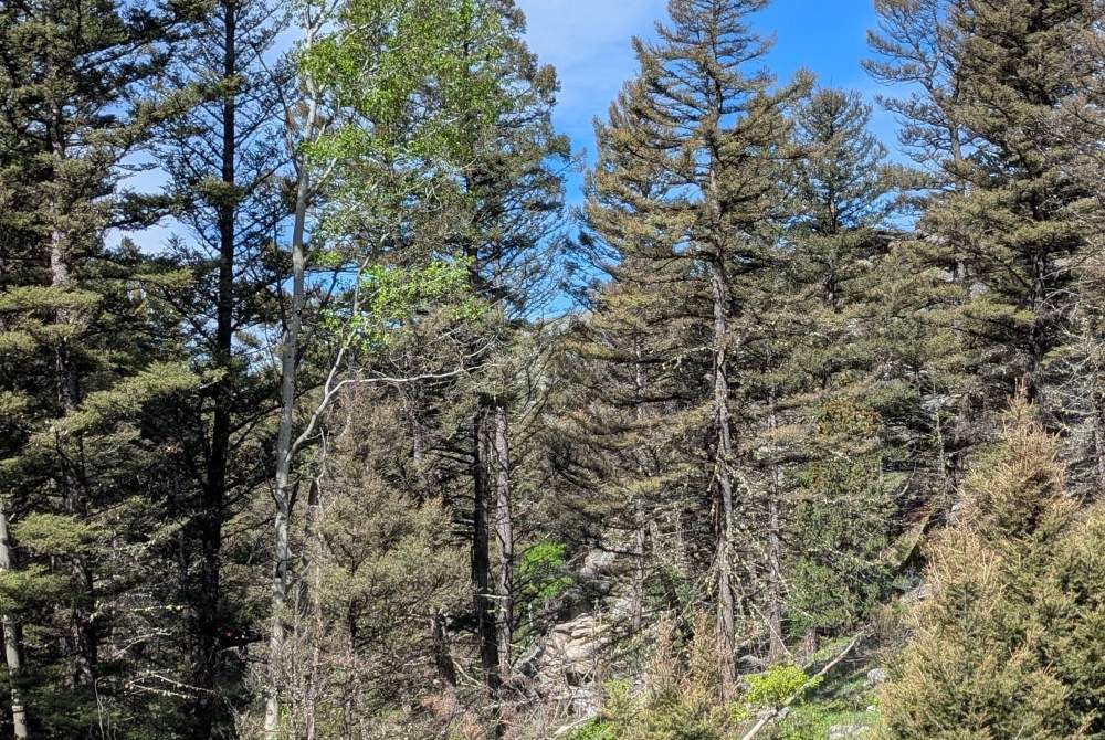
Our preparation started early as we needed to acquire high resolution data for the area to ensure accuracy. Prior to the event our data resolution in Montana was only 30m. We sourced 2m accuracy LiDAR from the USGS for the Ruby valley which we enhanced with 2m resolution tree canopy data from Meta.


Based on feedback from previous years about trees around the mine, we knew accurate tree data would be essential.

The data was loaded to the public system, CloudRF, weeks prior to the event and side-loaded to our offline SOOTHSAYER servers as GeoTIFF files within a data package.
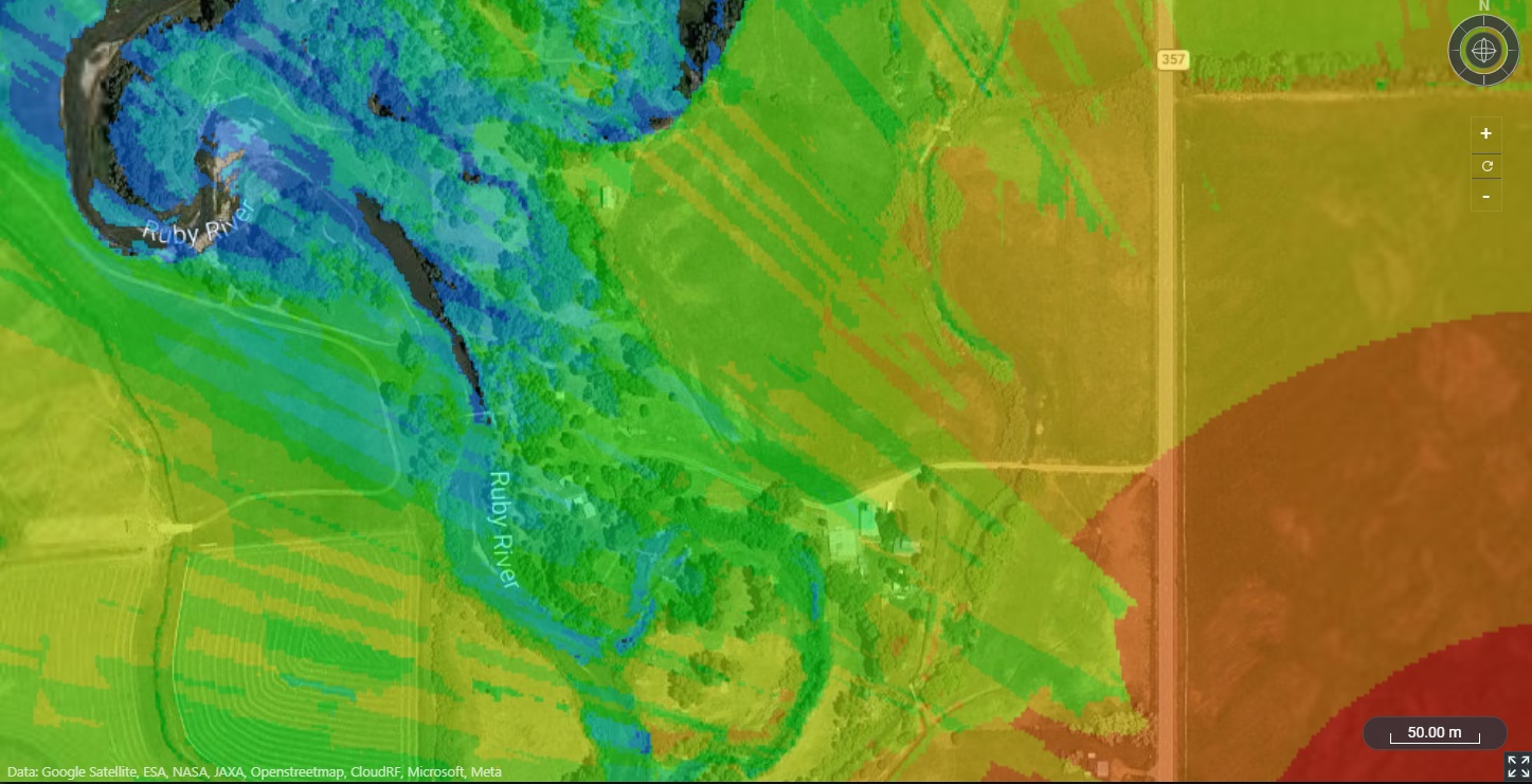
High resolution DTM and Tree canopy data in the Ruby Valley, MT

Equipment

We deployed with three offline SOOTHSAYER servers of varying size with several phones and tablets as clients:

  • A standard HP Z-Book laptop running Windows/Podman (RTX4070 GPU capable of 15.6 TFLOPS)
  • A Carnegie Robotics CardShark computer running Ubuntu/Docker powered by a portable USB-C power bank (Jetson Orin NX capable of 3.7 TFLOPS)
  • A Solace Communications Global Edge computer running Ubuntu/Docker powered by a larger USB-C power bank (Jetson Orin NX capable of 3.7 TFLOPS)

Additionally, The Global Edge computer was prepared with our Trellisware API script which interfaces directly with a donor radio to model live network coverage.

Site survey, Sunday

As we were headed to a new area, we were keen to know as much as possible about the terrain which for communications means noise as much as topography.
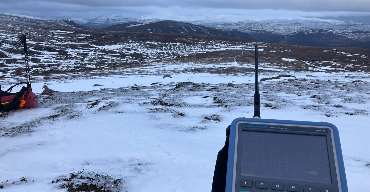
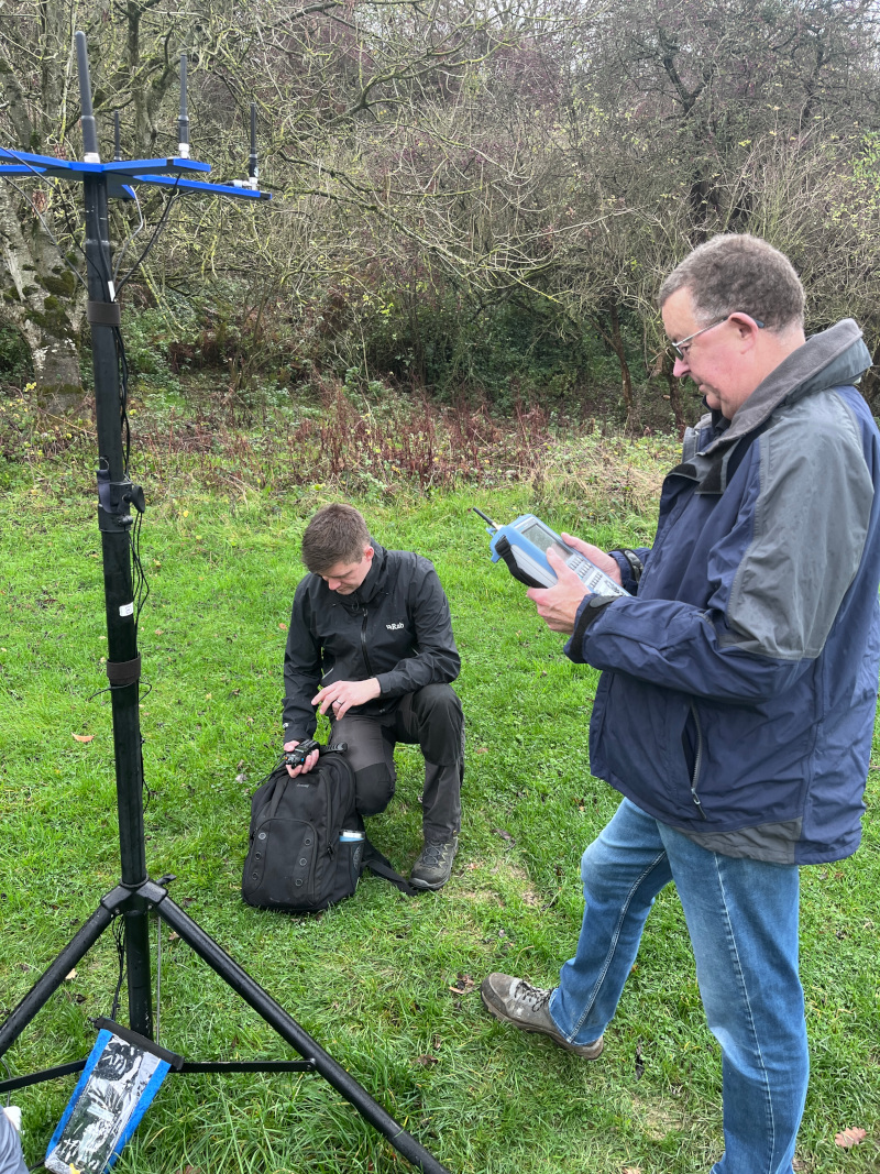
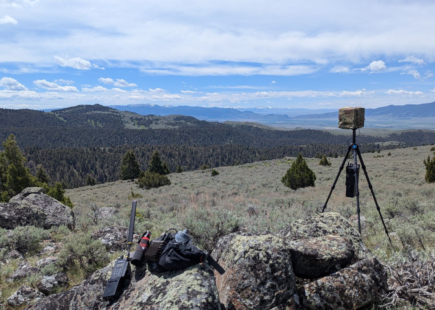
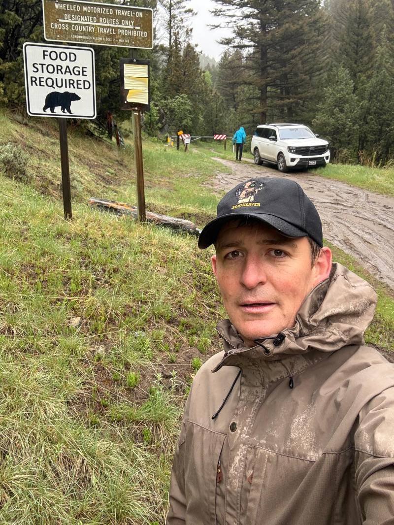
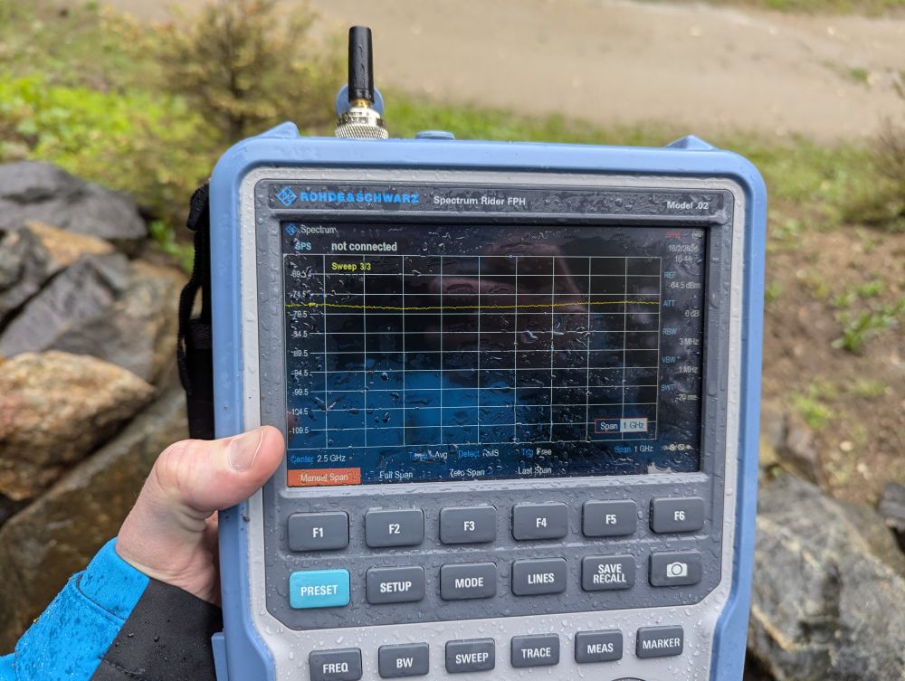
We took a spectrum analyser up to the mine site on a wet Sunday to check out the noise in the L and S bands and after a long insertion hike due to a closed seasonal access road we were satisfied to find there was no RF noise there.

The nearest noise source was a cell tower up the Ruby valley below which due its location was not able to serve the area of interest. We were therefore able to use the Johnson Nyquist formula with high accuracy to predict the expected noise floor for a given bandwidth.

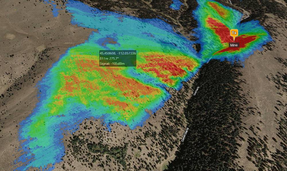
We modelled the Mine location with modest system profiles (low height/power) to see if we could identify any local relay opportunities. The mine was tricky as it was in a steep forest ravine so we stood at the entrance and observed where it could reach. This low tech study confirmed our modelling which highlighted a hill ~750m due west which just overlooked the mine and had excellent views across the Ruby valley to the south.
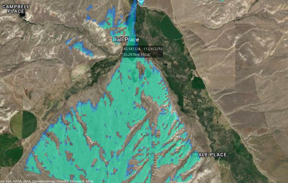
Using a mean site upon the hill within the painted coverage area we ran a second simulation with an extreme 40km radius to see where this could hit. We were pleased to see coverage on an embankment 35km down the ruby valley which was useful as the valley’s curved shape meant a relay would be required.

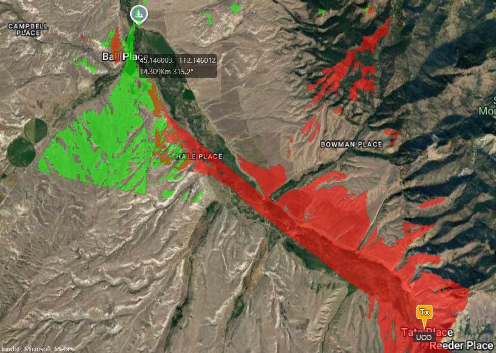
Next, we ran a simulation on the distant HQ location which revealed an area of mutual coverage. A plan was forming…

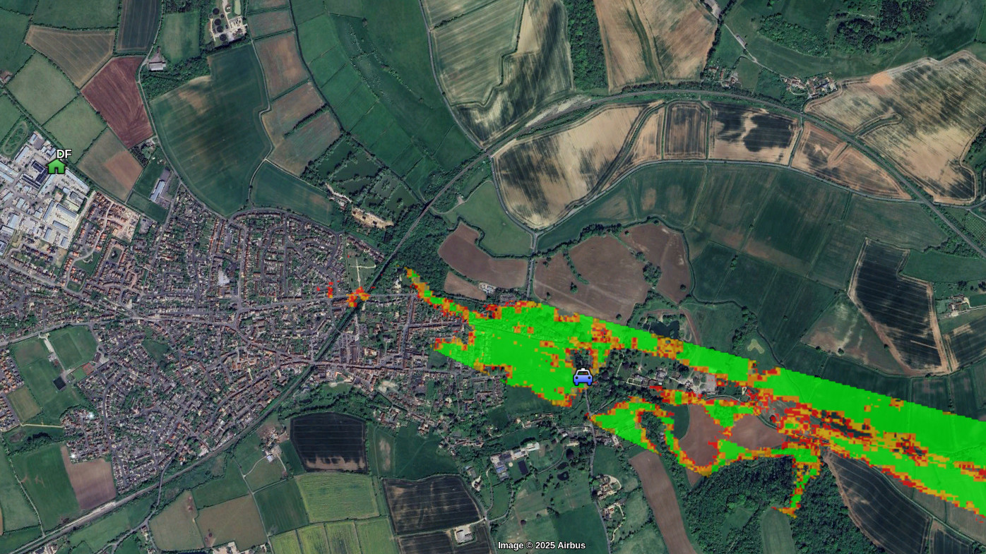
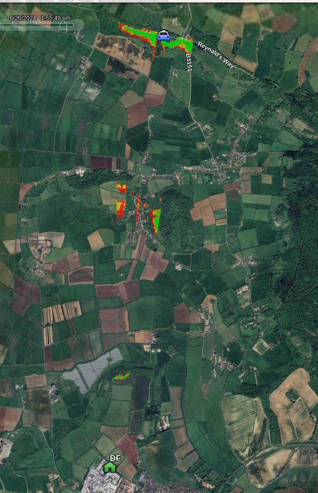
When running long range heatmaps, the resolution becomes diluted. This is necessary to remain within processing limits as whilst 16 million point calculations are available due to the large GPUS we have on CloudRF, they are impractical for a battery powered Jetson which must share its output over a radio network on ATAK. We also observed notable latency with fetching large KMZ files via the radio’s onboard Wi-Fi as it’s running an older 802.11 standard.

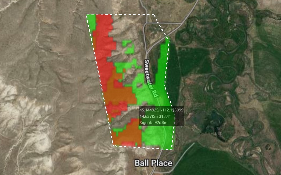
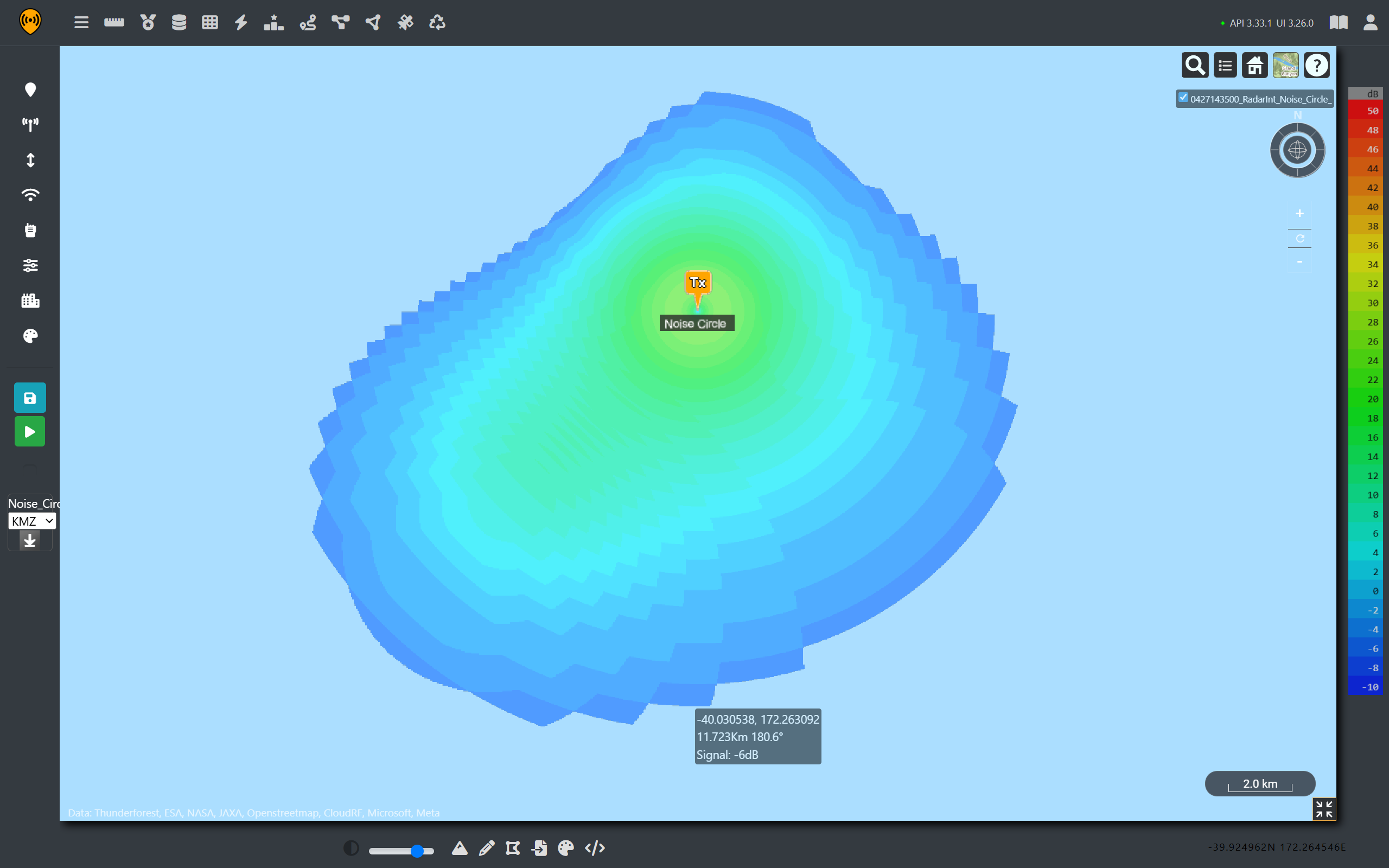
We used our plugin’s limit of 4MP which provides a high resolution result in a practical time of several seconds. Our solution to the ‘mountain repeater’ problem whereby a distant tower is serving a remote location is the bounds feature. This API parameter defines a polygon which focuses processing effort to increase speed and accuracy.

As you can see from the images, the difference the bounds feature offers is significant. It allows the simulation of high resolution at long distances which previously would have been impractical with a ‘big heatmap’.

We drove to the relay we wanted to use and were disappointed to find it was on private land which was time well spent none the less. As a result we identified a secondary site on a layby to the north which was the best we could do.
Setup, Monday

Our radio partner trusted our recommendation and deployed a Comrod ETAMs mast to the layby despite it not being recommended as one of the official repeater positions.
The first (15km) link back to the HQ was barely workable which aligned with the fringe heatmaps we had generated. The weak link was immediately made good by climbing the steep hill overlooking the HQ. The additional height cleared the Fresnel zone which was obstructed by trees and buildings in the valley.
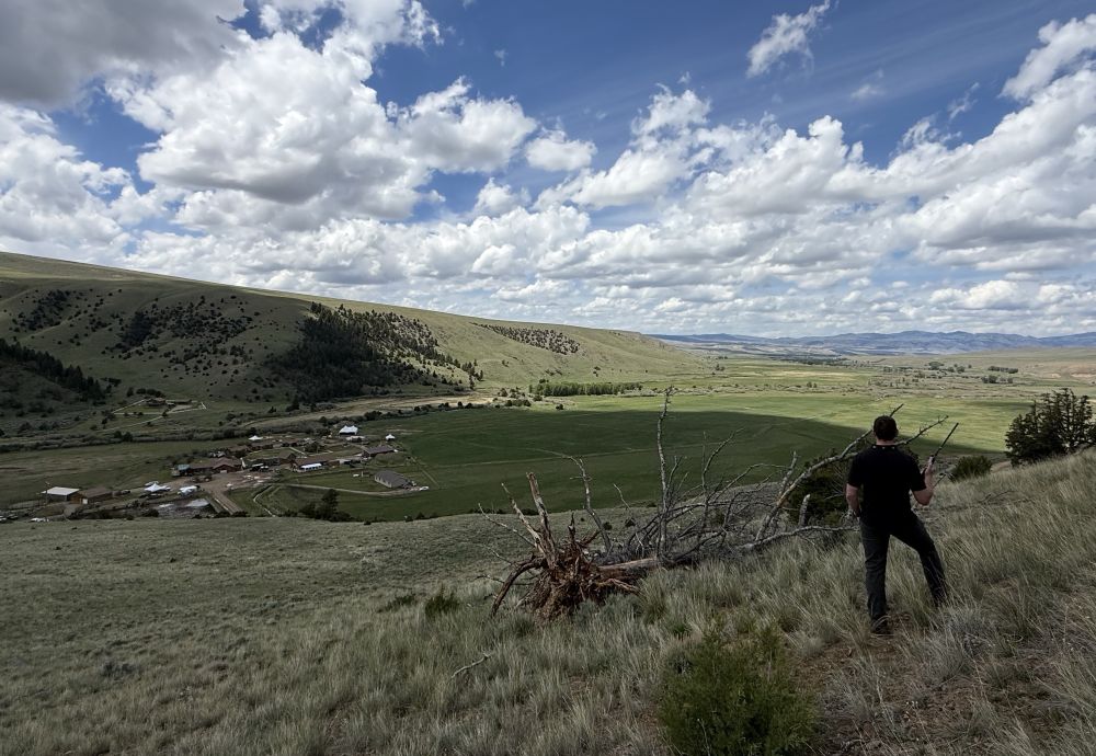
Improving the signal from a local hill

With the first link in, focus shifted to the long link to the mine.

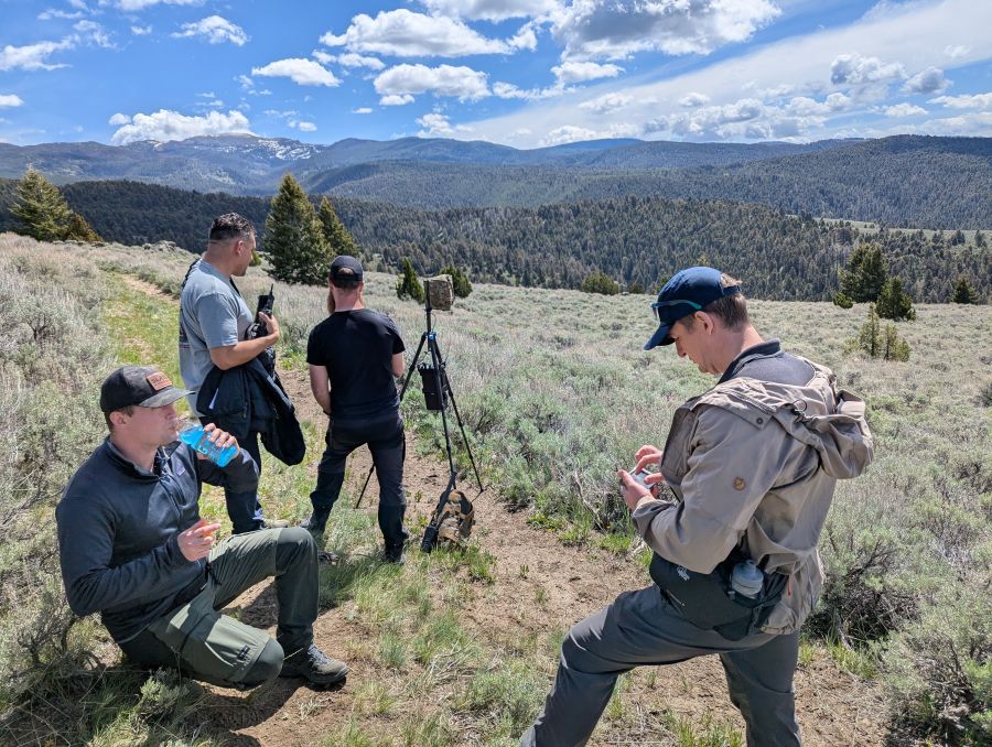
We drove up to the mine and headed out on foot to the exposed hillside we had identified from the mine. This was a steep and difficult route, in hot weather, with rattlesnakes and bears, which Alex H from Trellisware made no less than 5 times. Give that man a raise!

On the hill we used ATAK to navigate to the area on the track on the hill we had identified. This zone covered several prominent rocky outcrops which as we found were popular for sunbathing by snakes. Once in the zone, it became apparent that this would work as radios with low gain whips were connecting to the distant 35km relay. This link was boosted from workable to good, and fit for video, with the deployment of a Farfield Antennas APEX directional antenna.

Our relief at establishing communications was short lived as we were challenged to find a better spot. We used SOOTHSAYER on the CardShark server to simulate the midpoint relay to produce an updated layer. This layer was used to identify a better site nearby at a rocky outcrop on the hill. We relocated to the new site and were pleased to confirm a modest improvement to the link SNR. The scale in the change of location was minor given the 35km distance and the fact both sites had equally great views down the valley but the improvement was notable due to the shape of the convex hill and it validated accurate simulation over ‘looks good’.

During the excitement of closing the big one, we forgot to leave behind a radio at the mine to test the next link. This was soon rectified by a party which returned to the mine and confirmed a good link, which did not come as a surprise given the visibility from the mine and close proximity at ~750m.

A very satisfying radio check from the mine was heard at the HQ 50km away around the valley, over 3 links.
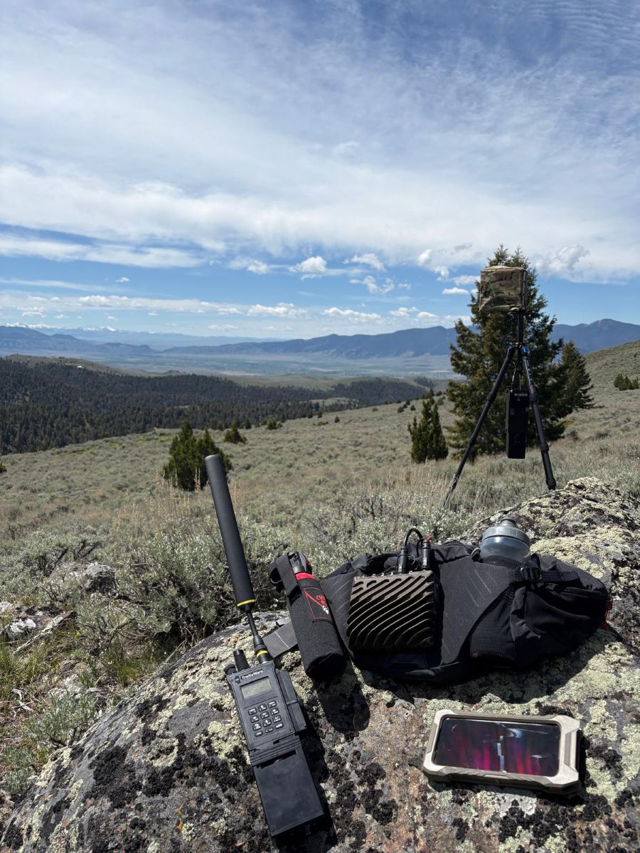
With the sites identified, the network was optimised with wired links between co-located relay nodes on alternative frequencies to increase throughput. There were other configuration changes higher up the OSI model also which are not covered here as we’re focused on establishing layer 1 only. The optimisations were designed to increase throughput and reduce latency to support both video and live UAS control.

Live coverage mapping

In our vehicle we kept our Global Edge server which had a higher endurance than the CardShark. This server was connected to a donor radio’s Wi-Fi access point as a client which enabled it to interact with the Trellisware API.

Our Trellisware python script fetches radio metadata to generate coverage heatmaps for the network using live settings including noise. This is presented as a network KML layer which is consumed by clients including ATAK.

We last demonstrated this in our office car park with our own TW-750 radios so it was exciting to use it on a mountain with a diverse network of different radios. We’re pleased to report it worked as designed after a tweak on the mountain to handle output from radios we’ve not worked with before. We’ve even heard a rumour the KML refresh may be lowered this year to support faster refresh rates, nearly 6 years after we requested this.

We also exercised the ATAK plugin’s Co-Opt function. This powerful feature allows any callsign on the map to be given a radio template which follows its position. As the callsign moves, the radio coverage moves. You can see a video of it on our youtube channel.
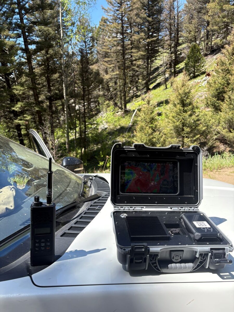
Global Edge server running SOOTHSAYER

Show time and interference

The network was scheduled to deliver a live video feed of a drone exploring the mine.

Despite a day of successful testing, leaving radios behind overnight in the mountains with wildlife and the elements meant unexpected issues were encountered which required local input to fix. On demo day an eleventh hour reset for the relay was promptly executed by Josh, who ‘hauled ass’ whilst observing local speed limits to get up the valley and save the day.

The live video was streaming well on schedule via a local radio’s WiFi access point until the production tent filled with observers… At this time, the congestion within the 2.4GHz ISM band increased and the impact became obvious as the video deteriorated and then failed. The irony of engineering a 50km muti-hop data network in the mountains and failing at the last 2m inside the tent was a learning point. In hindsight, a wired connection to the tablet would have been safer and people should listen to Peter.

The WiFi link self restored due to Automatic Channel Selection (ACS) and normal service resumed with live UAS video streamed over the RF link under the direction of the HQ.
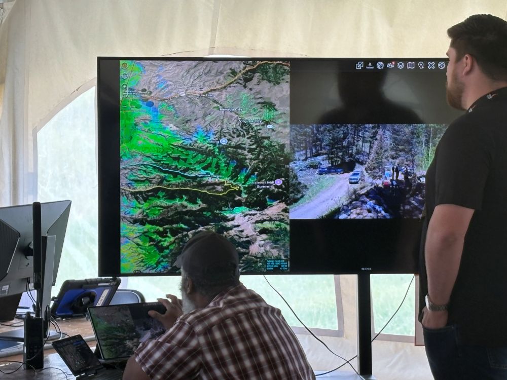
Live ATAK video relayed from the mine to the HQ

Summary

The event stress tested our capabilities to the limit, where it matters, and provided invaluable feedback we would never have found in a dozen trade shows or car park tests. We leave with very high confidence and a list of improvements and feature requests from the many customers and partners who we interacted with.

One of the most significant features will be the ability to expedite the site selection process for operators with a prompt to an LLM which can execute the multi-stage process of site selection using accurate radio templates. A lot of firms are chasing this AI dream but very few indeed have a mature, published, API to build upon.

We came prepared to model the inside of the mine using our 3D engine which was risky as we needed to acquire and then vectorise a large LiDAR scan from a robotics partner under a tight schedule. We acquired the model but hit formatting snags during the conversion to glTF so parked that task for another day. We did however produce a useful glTF to 3D tile script to present 3D models on ATAK which we will publish.

Despite the maturity, we’re still not elite enough to have our open source plugin listed on TAK.gov but as the push for published interfaces grows, we’re confident that sharing, not guarding, interfaces is the superior strategy for vendors serious about integration, more so in the age of AI. As more proof, we were pleased to see a shiny new plugin at this show that used our API with a radio API that was developed rapidly by a vendor without our knowledge.

Finally, for anyone still unsure if SOOTHSAYER works offline because our company has Cloud in the name, we can assure you it does as we do not own a Starlink and there is no cell coverage in the upper Ruby valley.

For more offline field tests see our Youtube channel.
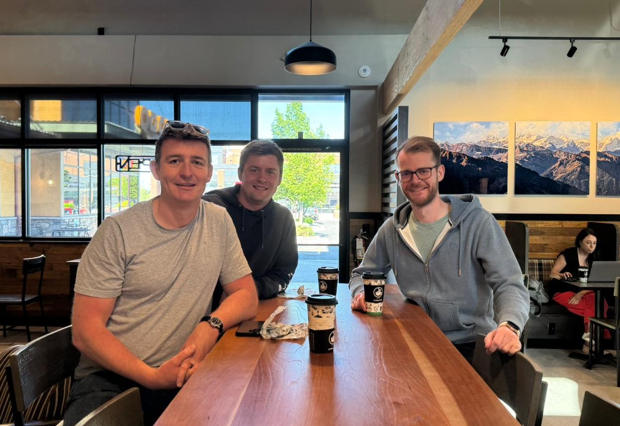
CloudRF celebrating like a privately funded company in City Brew Coffee, Bozeman

“CloudRF modeled propagation to help select relay positions before teams committed people and equipment to the terrain — validated by successful site selection, fewer hops, lower equipment requirements, and no wasted relay-site movements.”

Tough Stump Rodeo 2026 Executive Summary
Posted on

How a passing Warship took out a town’s Internet

Modelling Radar and Wireless interference in the 5GHz range

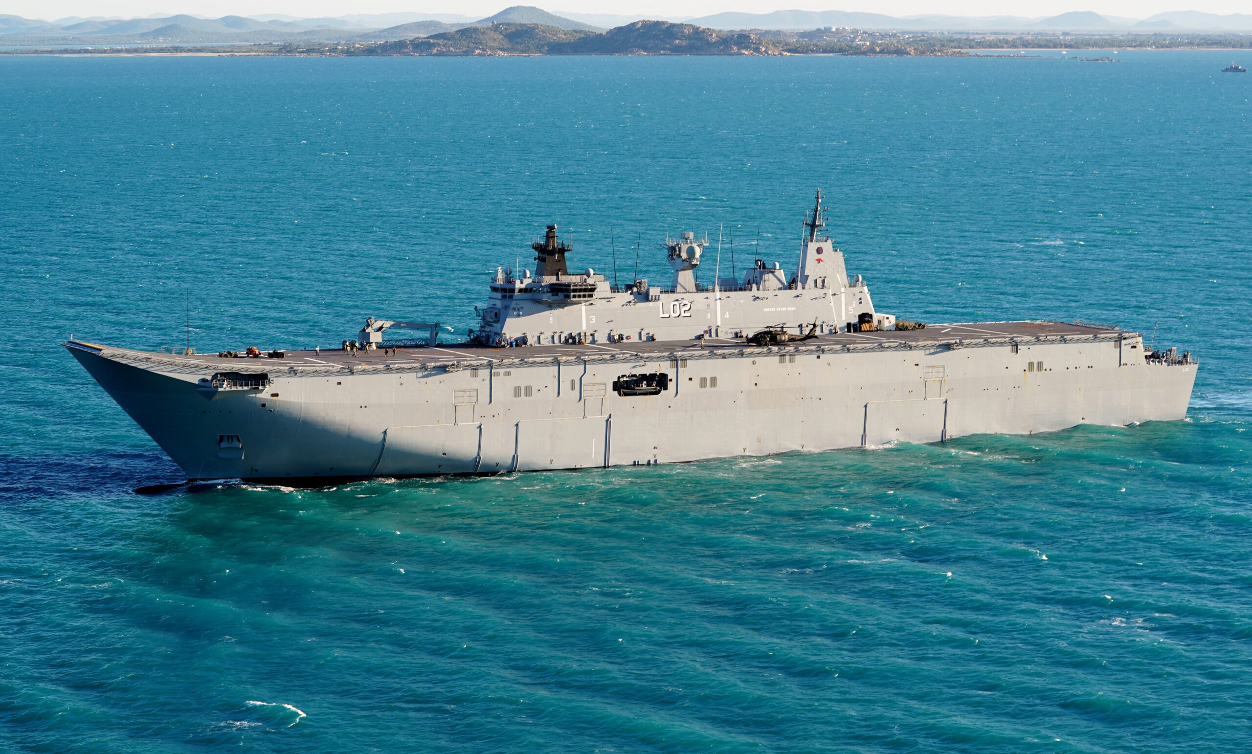
HMAS Canberra off the coast of Queensland, Australia (U.S. Air Force photo by 1st Lt. Joshua Thompson)

Background

In the early morning of the 4th of July 2025, the Australian warship HMAS Canberra sailed down the west coast of the North Island of New Zealand. It had its navigation radar on, surveying the sea for obstacles. At the same time, residents along the coast found their wireless residential and business internet failing. The story soon hit the local news sites which spread across the globe.

For most people, having their Wi-Fi supposedly jammed by a warship isn’t a regular occurrence so it’s not a surprise the story went viral. However, a lot of the explanations were incomplete and didn’t explain the science behind the issue.

Using the tools offered by CloudRF, we can recreate the events and learn how radar and wireless comms interact.

The Radar System: SAAB Sea Giraffe AMB

First, a clarification. Maritime navigation radar is not a monolithic category. Commercially, the most common bands are X-band (~9.5 GHz) and S-band (~3 GHz), both of which are regulated for civilian maritime use and appear on everything from fishing trawlers to container ships. Military vessels frequently also carry C-band systems (~5.5 GHz), which offer a useful engineering trade-off: better range and resolution against small surface targets than S-band, but with less atmospheric attenuation than X-band.

On board the HMAS Canberra, there is only one named C band radar, the SAAB Sea Giraffe AMB. From the brochure “The SEA GIRAFFE AMB is a medium range, multi-role surveillance radar optimized for detecting small air and surface targets with high update rate in all kinds of environments, including the littorals” which is ideal for transiting the rugged coastlines of New Zealand.

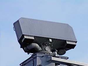
SAAB Sea Giraffe, image sourced from Radartutorial.eu

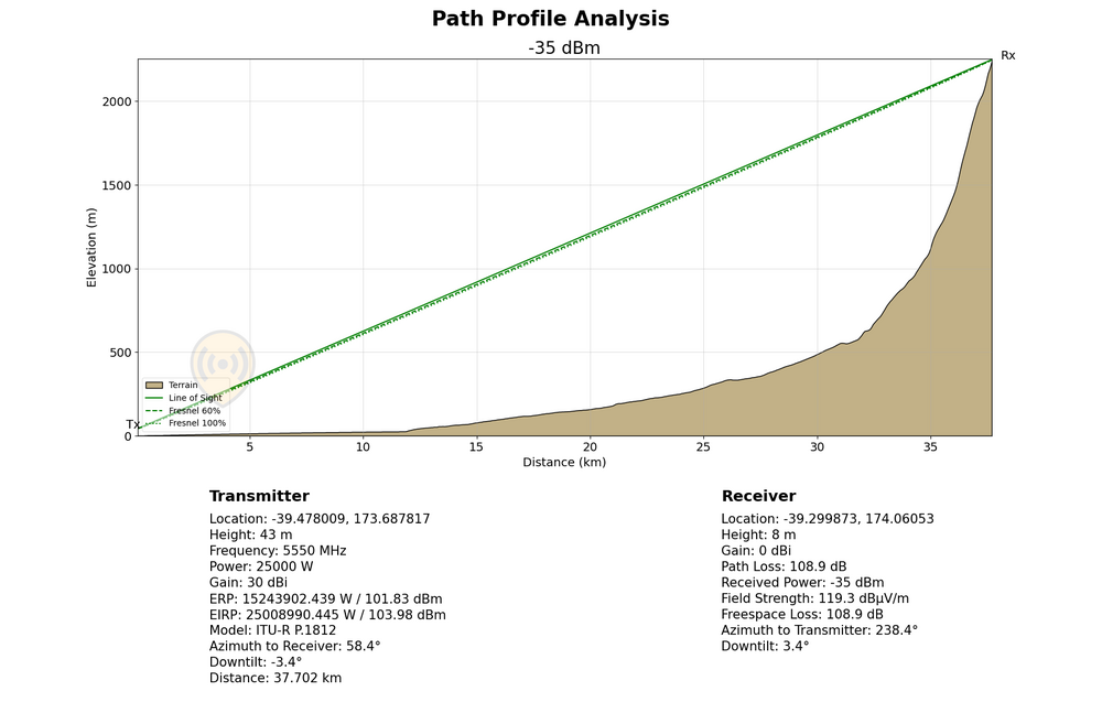
Naturally, full information on this system is not publicly available, so we shall have to try and source as much as possible and then estimate the remaining parameters. This will be saved as template in CloudRF and used for multiple calculations:

{
    "site": "SeaGiraffe",
    "network": "HMASCanberra",
    "engine": 1,
    "coordinates": 1,
    "transmitter": {
        "lat": -39.478009,
        "lon": 173.687817,
        "alt": 43,
        "frq": 5550,
        "txw": 25000,
        "bwi": 100,
        "powerUnit": "W"
    },
    "receiver": {
        "lat": 0,
        "lon": 0,
        "alt": 8,
        "rxg": 0,
        "rxs": -64
    },
    "feeder": {
        "flt": 1,
        "fll": 0,
        "fcc": 0
    },
    "antenna": {
        "mode": "template",
        "txg": 30,
        "txl": 0,
        "ant": 1,
        "azi": 0,
        "tlt": 0,
        "pol": "v"
    },
    "model": {
        "pm": 4,
        "pe": 3,
        "ked": 2,
        "rel": 50
    },
    "environment": {
        "elevation": 2,
        "landcover": 1,
        "buildings": 1,
        "obstacles": 0,
        "clt": "Temperate.clt"
    },
    "output": {
        "units": "m",
        "col": "GREEN.dBm",
        "out": 2,
        "nf": -94,
        "res": 60,
        "rad": 120
    }

First, we can estimate the transmission power to be around 25kW which in this case is going to be our peak power.

We will set our bandwidth to be 40MHz which gives us single digit meter range resolution, though this maybe too high for more general surveillance, these types of radars can adjust their bandwidth to help search for specific features.

We shall set our center frequency to be 5550MHz which places us comfortably within the C band range.

Our last two variables relate to our antenna. Radar antennas are naturally placed on a ships mast, and the HMAS Canberra has several. The exact height isn’t available, but we know the tallest point on the Canberra is “45cm below the Sydney Harbour Bridge” which is roughly 49m above sea level. Looking at the vessel, there are two towers which are shorter than the aft tower. We can see from photos of the Canberra that the sea giraffe is in the middle tower. By subtracting a few metres gives a transmit height of roughly 43m.

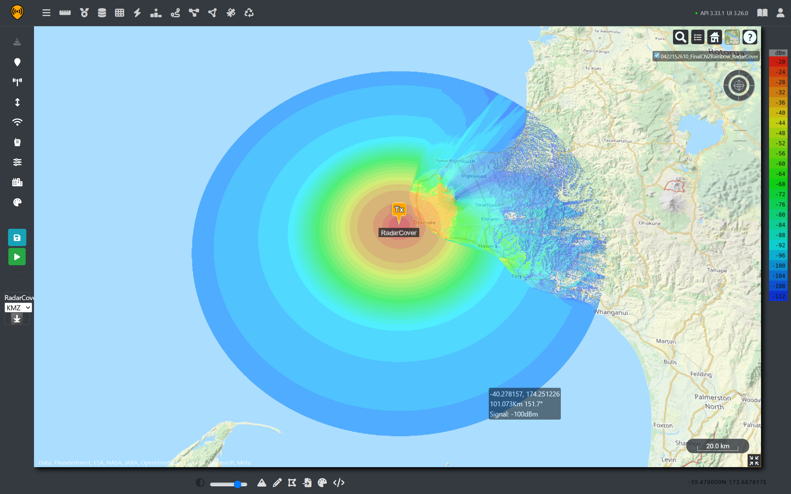
For the antenna itself, we will use it’s rotation our advantage and model the system as a dipole, giving uniform coverage in all directions. With the template set up, we can make a prediction of the signal strength around the ship and see the radar’s potential coverage which by design is significant.

Ship’s RADAR coverage

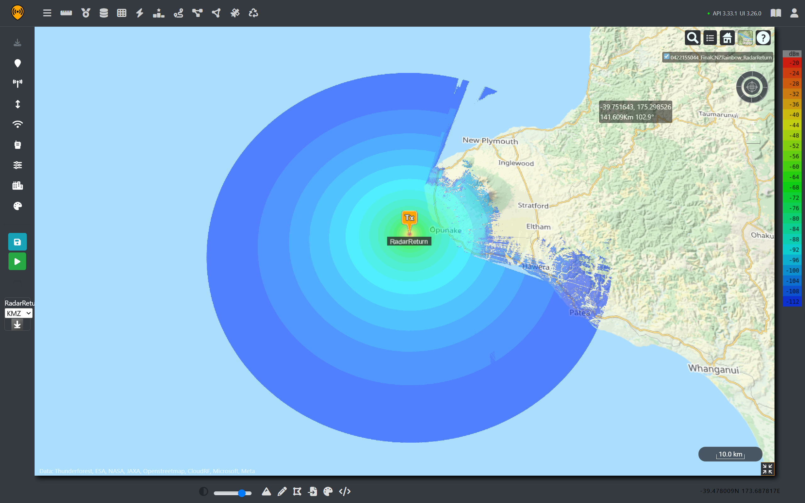
As we can see from the scale of the image, the HMAS Canberra’s radar signal propagates more than 150Km from the origin. However, as the signal must return to be sensed, we can use the radar model to give a rough indication of received power for a given radar cross section. In the image below an RCS of 10m2 at a height of 10m was used, giving much lower return values demonstrating why radar signals need so much more transmit power compared to regular communications.

RADAR detection range for a 10m2 cross section (ship or plane)

5G Fixed Wireless Access

On the other side of this situation, there are several privately owned and operated Fixed Wireless Access (FWA) networks providing rural communities internet access. In New Zealand, many WISPs utilise unlicensed RF spectrum under GURL licences. For a rural area at least, there are enough open channels and limited ranges that networks can dynamically operate around each other without causing significant interference issues.

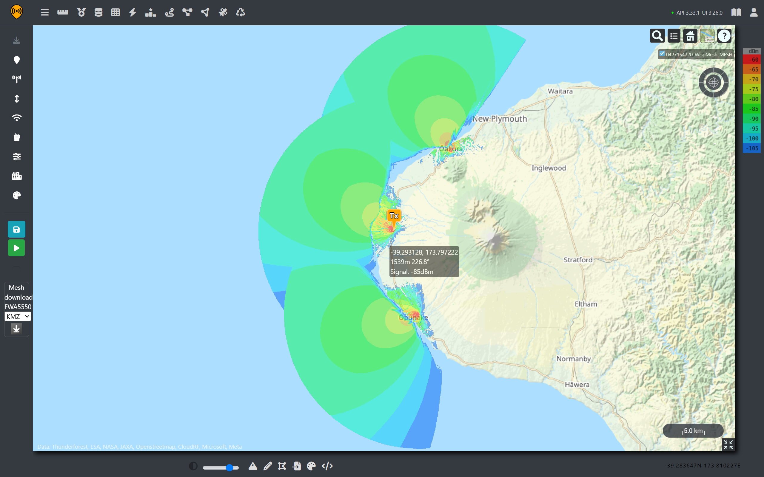
To develop an understanding how a network provides coverage, a fictional FWA tower is templated in Cloud RF and used to give wireless coverage over the small town of Opunake on the East Coast. We can use Radio Spectrum New Zealand’s licensing requirements to establish reasonable power, frequency and tilt requirements. We set our receiver at 5m to represent a rooftop in the nearby towns.

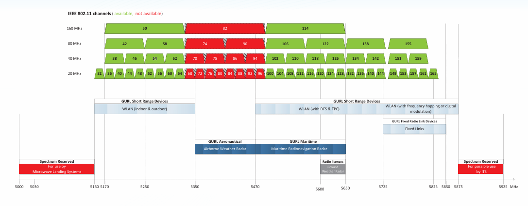
For frequencies we can implement Radio Spectrum Management New Zealand’s FWA allocation depicted below.

5G FWA template

{


    "site": "Site-A",

    "network": "NZ-WISP",

    "engine": 1,

    "coordinates": 1,

    "transmitter": {

        "lat": -39.283647,

        "lon": 173.810227,

        "alt": 22,

        "frq": 5550,

        "txw": 0.01,

        "bwi": 40,

        "powerUnit": "W"

    },

    "receiver": {

        "lat": 0,

        "lon": 0,

        "alt": 5,

        "rxg": 23,

        "rxs": -105

    },


    "antenna": {

        "mode": "template",

        "txg": 23,

        "txl": 0,

        "ant": 3587,

        "azi": 310,

        "tlt": 1,

        "pol": "v"

    },

    "model": {

        "pm": 4,

        "pe": 2,

        "ked": 2,

        "rel": 50

    },

    "environment": {

        "elevation": 2,

        "landcover": 1,

        "buildings": 1,

        "obstacles": 0,

        "clt": "Temperate.clt"

    },

    "output": {

        "units": "m",

        "col": "LTE.dBm",

        "out": 2,

        "nf": -90,

        "res": 20,

        "rad": 30

    }

}

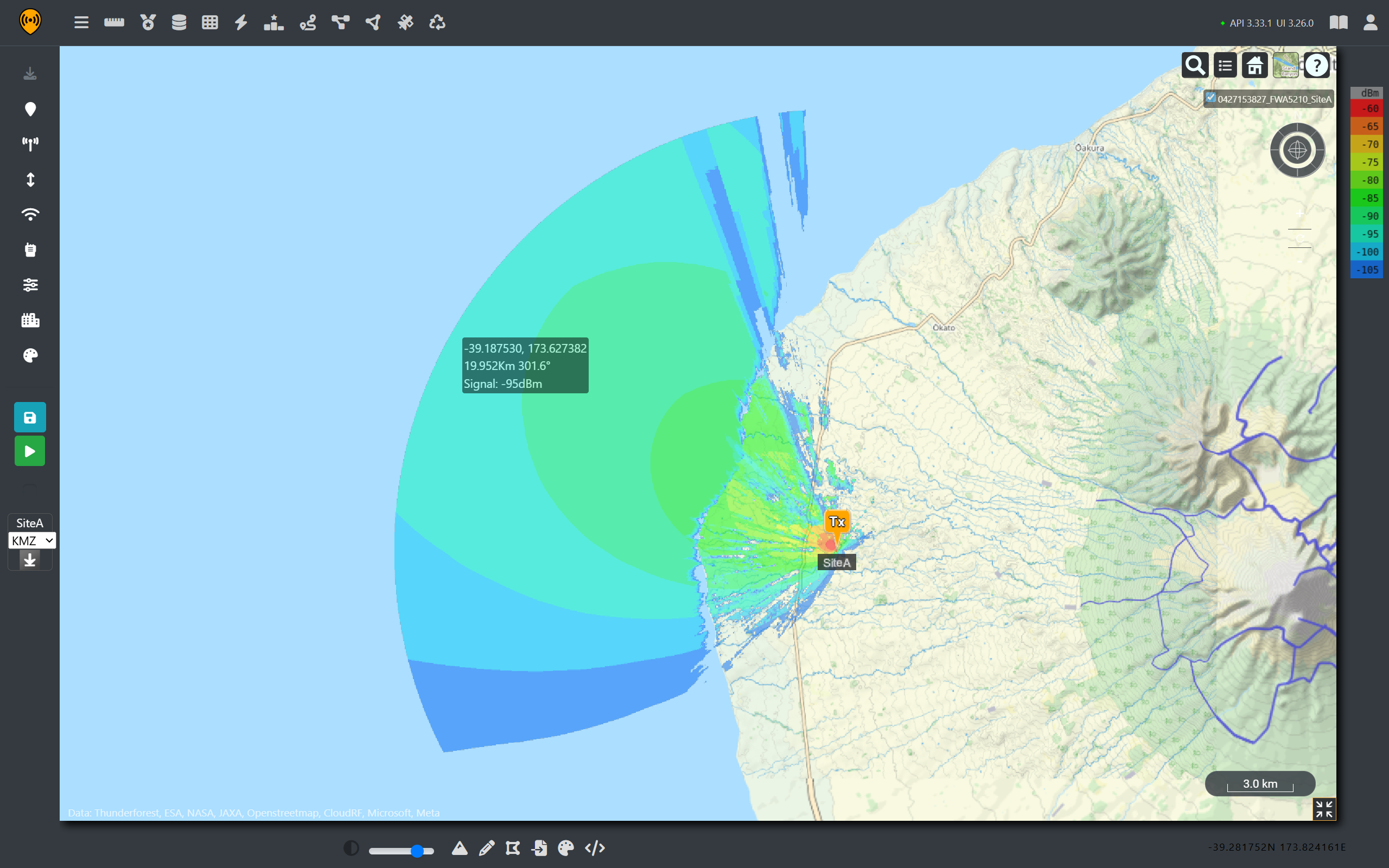
Selecting channel 110 sets the center frequency to 5.55GHz, and a coverage map can be created for the fictional site.

Fictional hillside FWA site on NZ coastline.

From the coverage prediction, we can see that the relatively low power WISP is still receivable from nearly 20Km away with a clear line of sight for a 40MHz link. So, for any coast facing towers, there’s a good chance their signal can be detected offshore well past the intended service range.

Fictional 5GHz FWA network

Dynamic Frequency Selection

As part of the licence requirements, radios using these bands are equipped with Dynamic Frequency Selection (DFS). This is an intentional safety mechanism recommended by the ITU to prioritise and protect Maritime radio navigation systems. The goal is to prevent interference by triggering a shutdown upon detecting radar pulses. The priority is to protect the radar picture which is safety critical.

Above a threshold, a received pulse will cause the wireless device to switch to a different frequency or shutdown it’s radio. It will listen out until it can no longer detect radar pulses before returning to that frequency and transmitting again so is performing automated de-confliction.

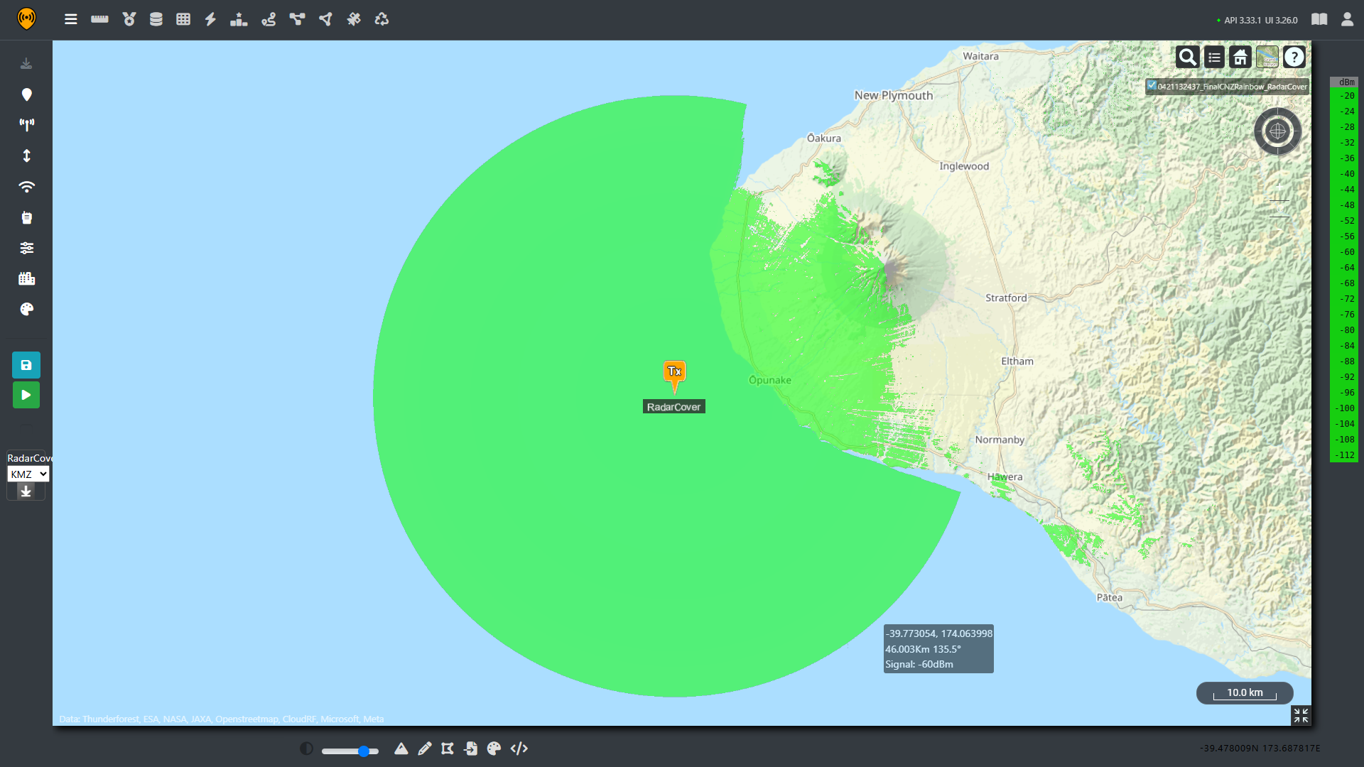
For our FWA systems, the threshold is set to -64dBm from a radar, received by a reference dipole with 0 dBi gain which is very easy to set up in Cloud RF by adjusting receiver sensitivity up to -64dBm and then remapping the coverage. In the image below, the areas in green represent a radar signal above the threshold that will trigger DFS.

Coverage at the threshold which will trigger DFS interference logic

As we can see, the radar signal easily covers the coastline and extends deeper into the mountainous areas. However, this is just a fixed location and not representative of the dynamic coverage of the moving platform.

Estimating the Full Extent of the Outage.

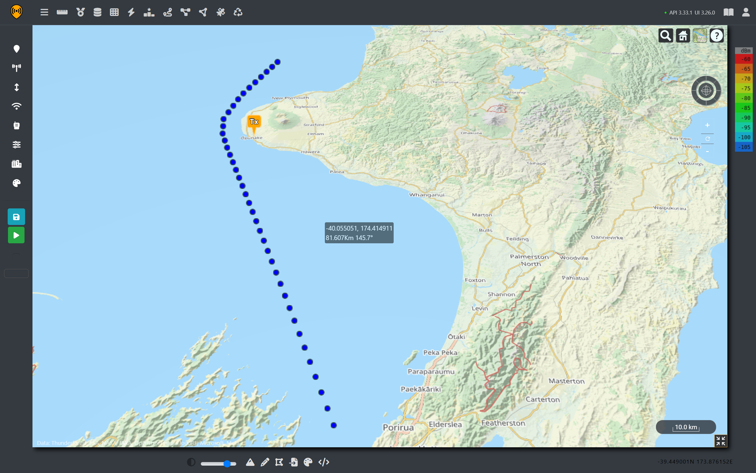
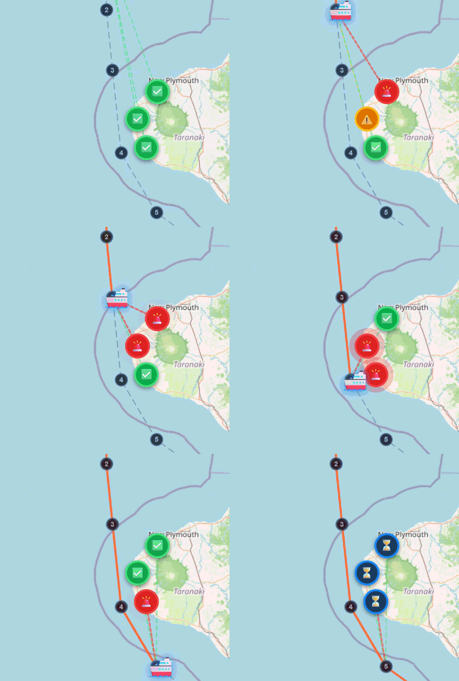
Rather than picking and analysing a single spot, we can recreate a similar course sailed by the HMAS Canberra and then use points along this track to build a comprehensive understanding of the impacted coastline.                                                                      

We know that the ship sailed down the west coast of the north island before heading into the cook straight on the way to its destination in Wellington. It’s not clear when the ships radar was switched to a different frequency and it is not possible to get historic coordinates like commercial shipping so likely course has been chosen.

Simulated course for the ship

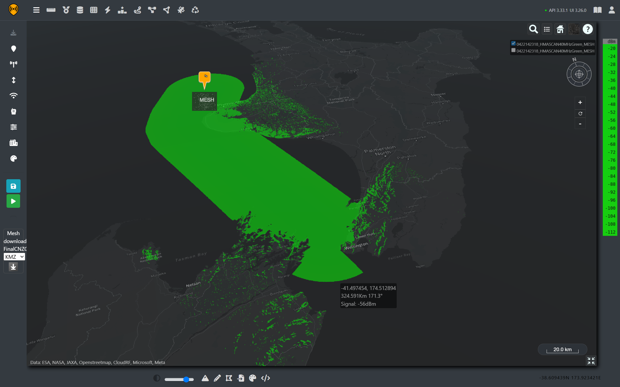
Using automatic processing, we can use the radar template to efficiently model coverage for each point and then use Superlayer to combine these results into a single layer.

Super layer for the moving RADAR

Using our templated radar, we can see that the entire coastline on the West Coast is a above the power threshold that would trigger DFS. We can also see that northern coastal and mountainous areas of the South Island. This aligns with the reported outages and also shows affected areas which may not have made the news.

On the west coast, we can see that the gentle slope up from the coast towards Mt Taranaki offers little obstruction to the radar signal.

From the coverage maps it is safe to conclude that the outage was caused by the DFS triggers rather than physical interference on the antennas. It was an inconvenience for the affected businesses and customers but an effective demonstration of spectrum co-existence technology working as intended.

For many readers of the subsequent news articles, it was the first time they had learnt that a ship can disable internet access, and it’s a standard baked into radio equipment.

What if there wasn’t DFS?

When viewing these images, it might be tempting to ask the question, “Why does this radar system need protecting? And what would happen to the FWA network if DFS wasn’t required?

To do that, it is necessary need to investigate both emitters to see how the two networks could interfere with each other.

Radar Signal Interference on the WISP.

To establish the interference of one network upon another is a straight forward task with the interference tool. However, before we can jump straight into the analysis, we need to make sure we are comparing apples to apples.

To begin with, radar signals are typically circular polarised. However, our FWA is vertically polarised so we will have some polarisation loss which will be estimated at -3dB.

Additionally, the centre frequency our radar system and bandwidth is not always the same as our radio channels, we will need to compare across the range of channels to see how the radar system affects adjacent channels rather than just co-channel interference.

Referring back to the RSMNZ chart, we can see that many channels are varying bandwidths. For this analysis, we will focus on the 40MHz 802.11 channels.

802.11 Channel NumberCentre Frequency (MHz)
1025510
1105550
1185590
1265630
1345670
1425710

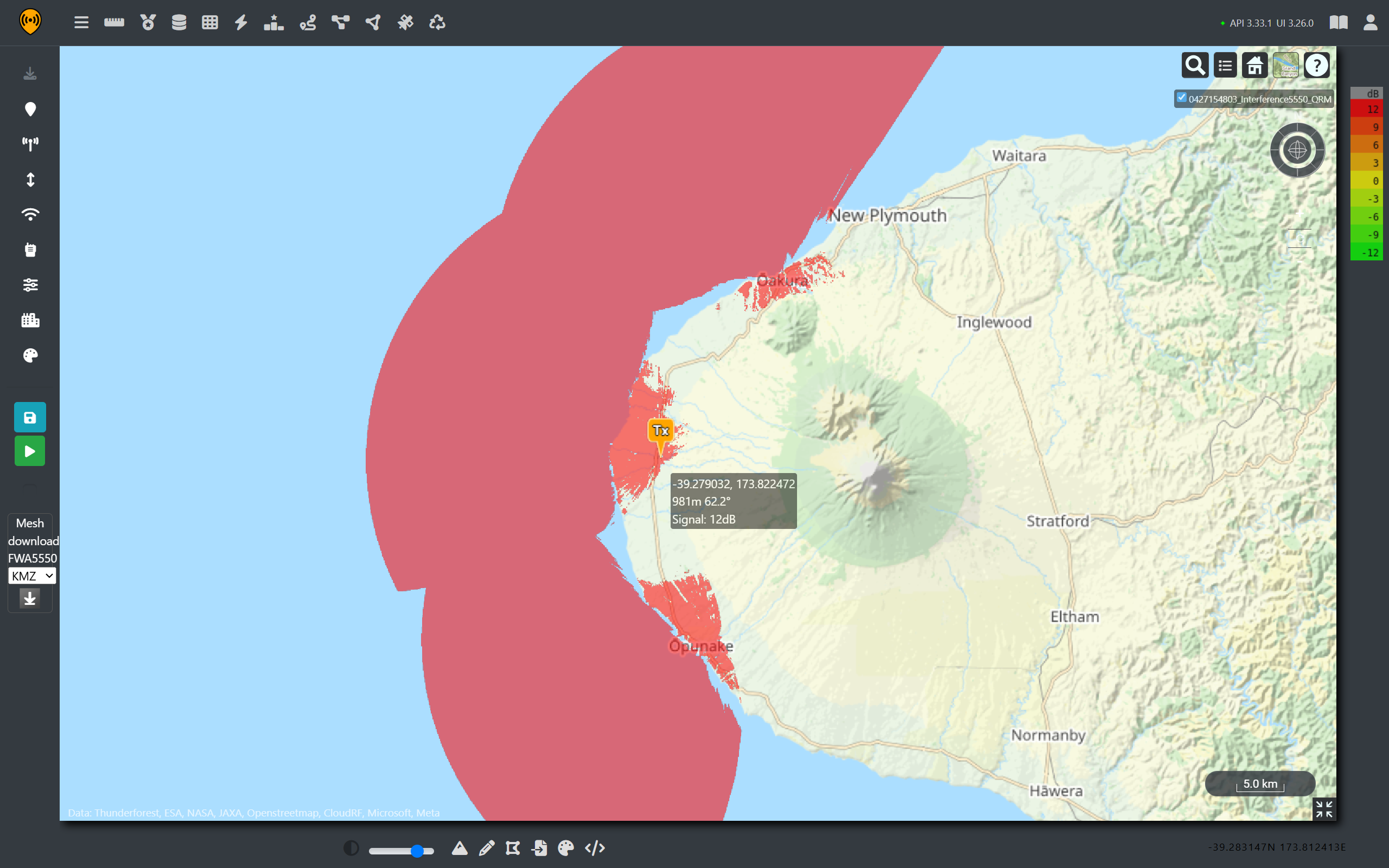
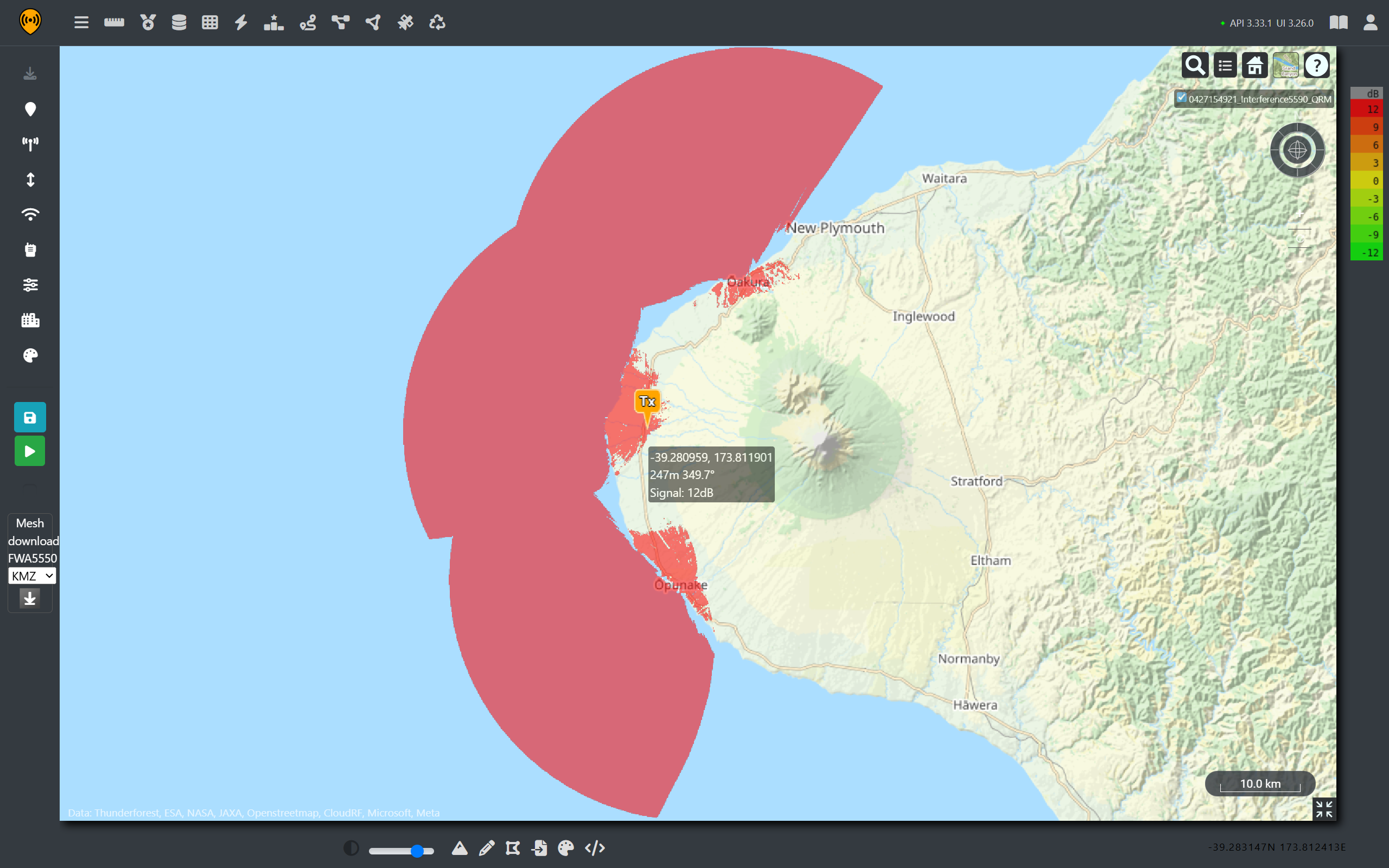
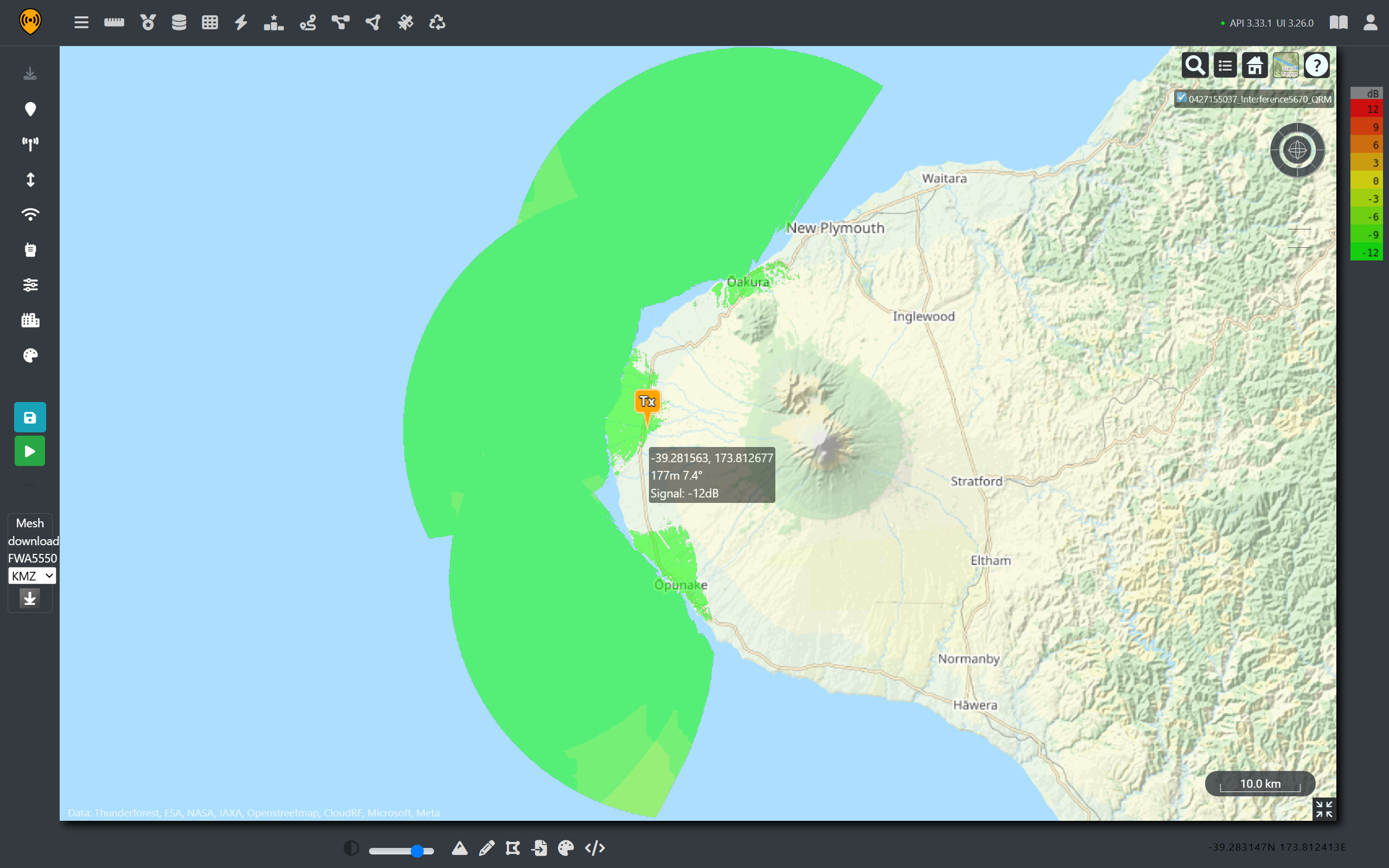
Using our FWA templates, we can quickly produce coverage maps and then use the interference tool in Cloud RF to see how the ship’s radar will impact connectivity on these channels of interest. Recalling that we are using a 40MHz radar signal centred at 5550MHz, we would expect to see interference within the range of 5530-5570MHz. This would overlap with channels 102 and 100, leaving the rest of the spectrum clear.

By using the interference tool, we can see that the simplistic assumption was only half-right and the relative strength of the radar signal has caused interference outside of it’s 40MHz bandwidth. Adjacent channel interference can still be observed up to 5630MHz before it drops away leaving channels 134 and 142 clear.

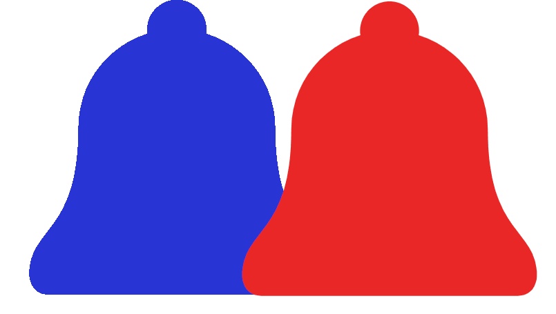
Signal power is shaped like a bell and is wider in practice than on paper.

Adjacent bells overlapping

As the radar bandwidth was assumed to be 40MHz, there is a possibility the actual SEA Giraffe could have used a wider bandwidth which would have caused wider adjacent channel interference, leaving none of the 40MHz 802.11 viable. So given the high levels of adjacent channel interreference we can safely say that without DFS, these WISPs would still be dealing with a significant outage until the ship had passed.

WISP Interference on the Radar Screen.

If the radar is so powerful, why is priority given to it compared with low power home networking equipment?

For that reason, it is worth looking at the effect of interference on a radar return. First and foremost, we need to understand the purpose of the radar is to aid navigation. Radio navigation is critical for detecting hazards when visibility is poor. For a military ship, particularly a helicopter carrier, surveillance and coordination of close airspace is also a key task.

Measuring interference is not easy as the exact relationship between the wireless transmission and the radar receiver is complex however we can model some educated assumptions to show the potential effect.

First, not all the power from the coastal signal will be absorbed by the radar antenna due to polarisation and what is makes it to the radar screen will be further attenuated by the receiver’s processing gain as the radar will use spreading codes, beamforming and other techniques to improve selectivity and mitigate interference. To model them, we’d need very detailed information on the Sea Giraffe which is not publicly available.

What we can observe, however, is the rise of the noise floor due to the addition of WISP transmissions around the ship and this will impact the signal-to-noise ratio (SNR) before signal processing.

First, we will use a FWA channel that is entirely within the bandwidth of the radar signal to keep spectral density simple. For this case we will use channel 110 at 5550MHz.

The noise floor is given by the combination of the radar’s thermal noise, the power of the FWA signal and other sources. Noise is computed using the signal power divided by Boltzmann’s constant.

Nfloor=kTB+PWISP

ΔNfloorPWISP(in-band)kTB

ΔNfloor(dB)10log10PWISP(in-band)kTB

As the radar noise floor is relatively constant, by using Cloud RF, we can generate received power predictions and then use the noise database feature to visualise the effect of a changing noise floor on radar return coverage.

We will use another fictional FWA site that is pointing out along the coast, providing coverage to a coastal town. From this tower, the signal propagates beyond it’s intended audience and is received by the ship’s antenna.

To address the change from vertical to circular polarisation, we can factor in a -3dB loss.

Ship’s course traversing a local wireless network

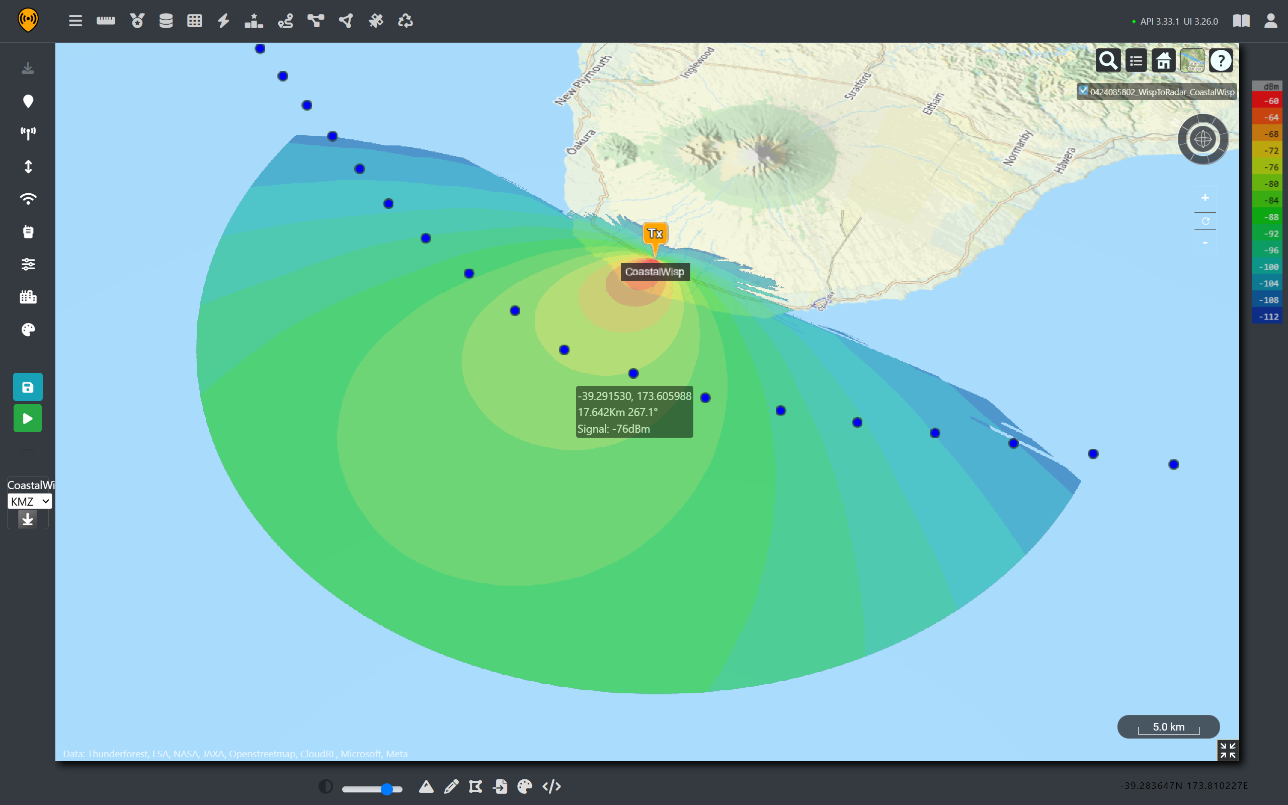
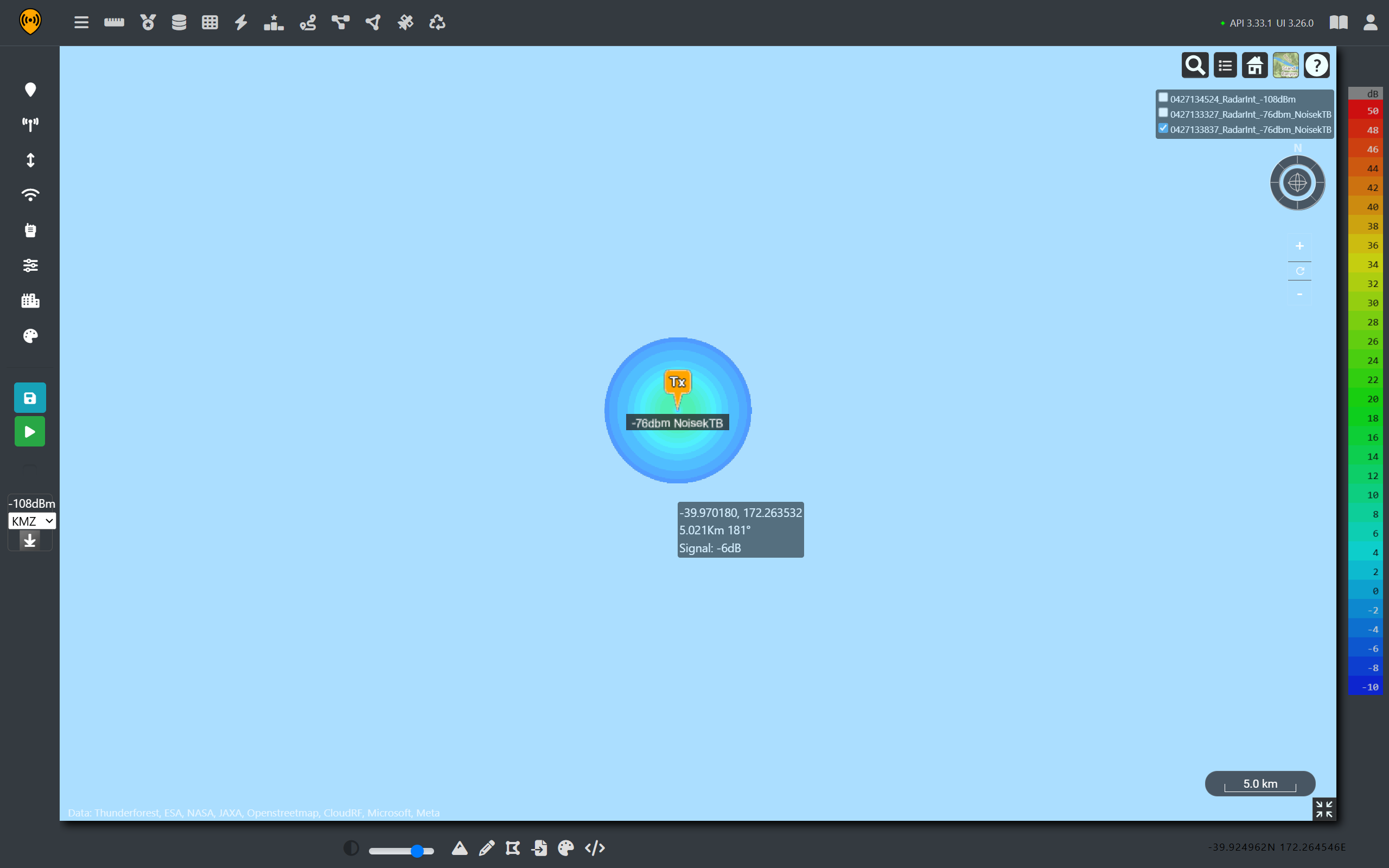
At our reference points, we can see that the ship travels through the FWA coverage, which peaks at around -76dBm despite being over 16km away from the receiver. This is because our radar antenna is elevated and it has a high 30dBi gain. As both systems are working on channel 110, all of this received power is in band for the radar and adds to the noise floor.

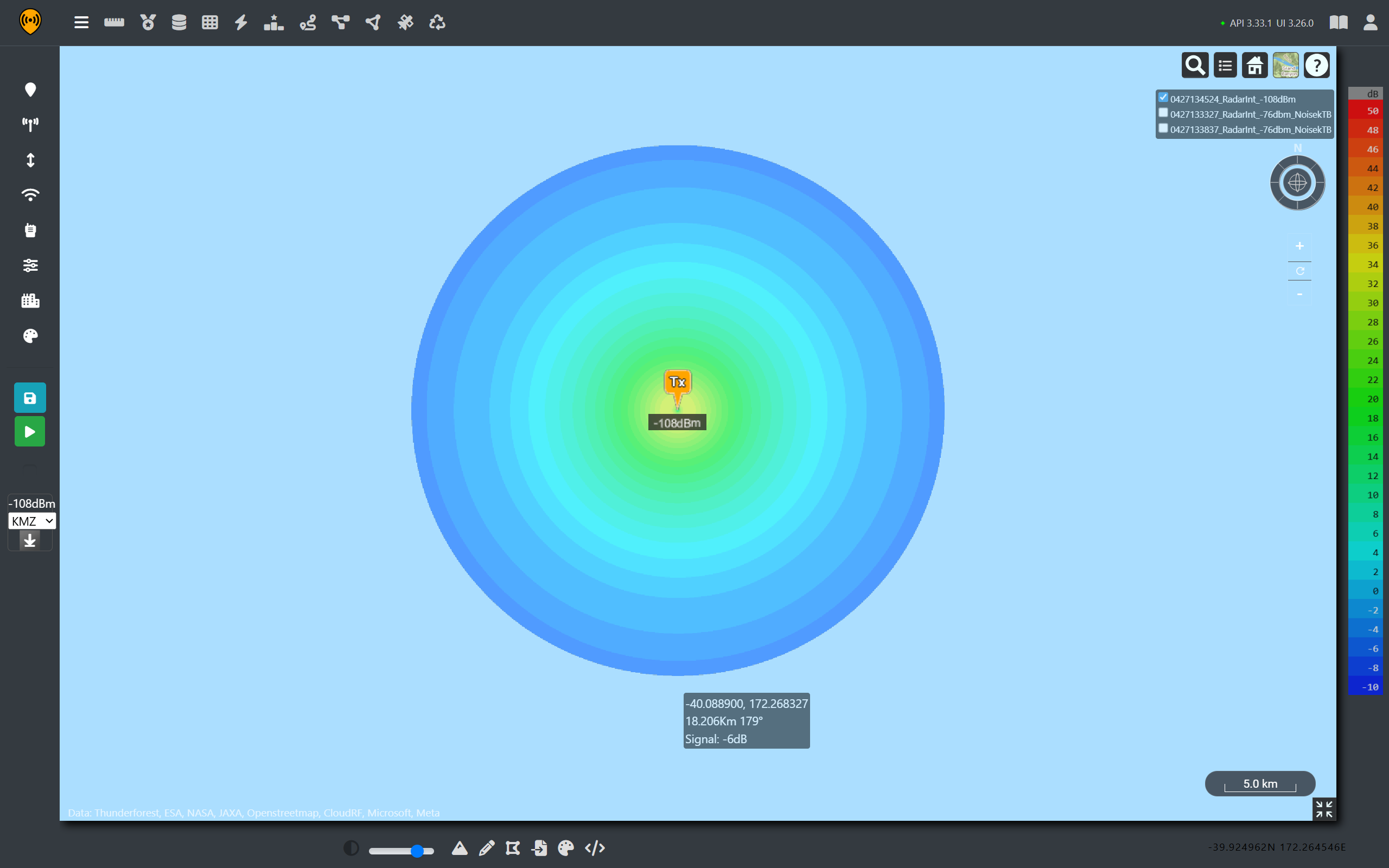
With a value for WISPs sorted, we can calculate the Radar Thermal Noise Floor at 40 MHz.

N = kTB = 1.38×10⁻²³ × 290 × 40×10⁶ = -108 dBm

And then converting to mW we can see that our new noise value is dominated by our WISP signal due to the orders of magnitude in difference.

Noise SourcesPower (mW)
Thermal noise (-108 dBm)1.585 × 10⁻¹¹
WISP in band (-76 dBm)2.512 × 10⁻⁸
Combined≈ 2.512 × 10⁻⁸ (-76dBm)

For a simple SNR equation, this much noise will lead to a drastic reduction in detection range. In reality, the Sea Giraffe will have front end filtering and signal processing techniques built in to significantly boost it’s signal ratio and maintain a clear picture. It is also important to note that this interference will only be coming from one angle, which makes it’s effect asymmetric.

From the different coverage plots, we can see that varying noise sources change coverage significantly and as RADAR is a directional array, a blind spot can be directional.

We can see that there is potential that increased noise in the C band could lead to a notable reduction in radar picture accuracy which presents a danger to maritime navigation, which has priority.

From the analysis, it is clear that the DFS system functioned as intended. It kept the ship’s navigation systems safe from interference at the cost of a temporary disruption for the coastal communities.

To prevent this happening, visiting warships could be given spectrum assignments clear of civilian infrastructure, or could signal their intentions in advance to local spectrum authorities. Vigilant spectrum surveillance could also provide early warning of anomalies which could be communicated to local spectrum users.

Coastal interference demo

Because we’ve leveraged the Cloud RF API and made templates, we can package our multi-step static analysis into a dynamic and simple tool. Using everybody’s new team member, Claude, we have published a simple tool which can demonstrate the signal strength for a ship’s radar as received by a coastal network.

Explore the tool here: https://cloud-rf.github.io/CloudRF-API-clients/slippy-maps/radar_interference_demo.html

Animation from the coastal interference demo

References

HMAS Canberra https://www.dvidshub.net/image/6755556/us-special-operations-australian-navy-accomplish-combined-black-hawk-deck-landings

HMAS Canberra Capabilities, https://www.navy.gov.au/capabilities/ships-boats-and-submarines/hmas-canberra-iii

SAAB Sea Giraffe AMB, https://www.radartutorial.eu/19.kartei/07.naval/karte038.de.html

HMAS Canberra accidentally blocks wireless internet and radio services in New Zealand | RNZ News

Australian navy ship accidentally blocks internet and radio across parts of New Zealand | Australian military | The Guardian

Posted on

Enhancing Radio Direction Finding with RF simulation

Background

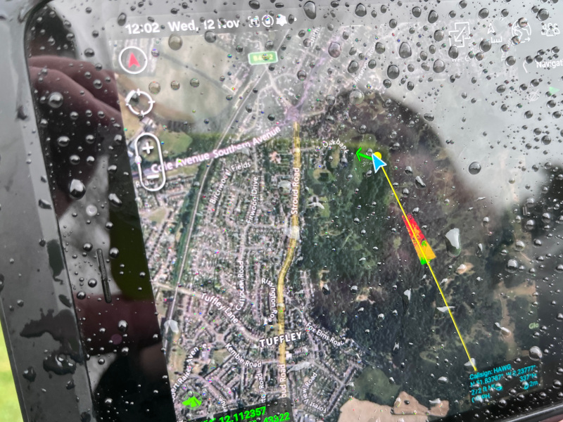
Radio Direction Finding (DF) is the art of determining the location of an emitter and is used in search and rescue, coastal surveillance, law enforcement and defence. There are different techniques using power and phase but the output for a single sensor is normally a Line of Bearing (LoB) which points towards the emitter.

If you’ve ever seen DF depicted in marketing or an info-graphic, you’ve likely seen three geometrically distributed sensors surrounding an emitter which produce a high accuracy position fix (PF) where their lines of bearing converge.

In the real world, DF systems are expensive and require specialist training so are in short supply. It is far more common for these systems to be used in isolation so operators must determine an emitter’s location with a single LoB and a map study. For powerful signals, the search area could be vast.

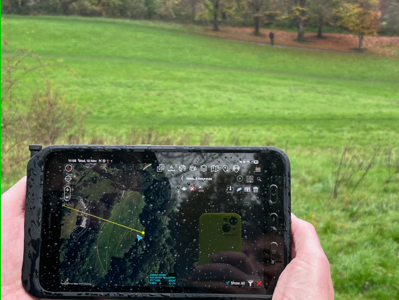
A Line of Bearing displayed on ATAK

Guessing the signal power

For a signal to be tasked for DF, it’s frequency is already known. With signal classifiers increasingly integrated into receivers, and now even open source, the signal type may well be known which helps answer a key question: what is the signal’s transmit power?

When a new signal is detected, it could be in the room next door or in the next county. Knowing the signal type and ideally the hardware is key to estimating the distance, as you can lookup the possible power levels from a data sheet.

A portable radio has variable power levels: For a DMR radio with low and high power at 0.1W and 4W these can be put into a basic path loss model to determine the possible distance. Using the Friis reference model with a detected signal of -80dBm for example, a 1GHz signal could be 2.4km or 15km away in free space.

Spectrum analyser up mountain
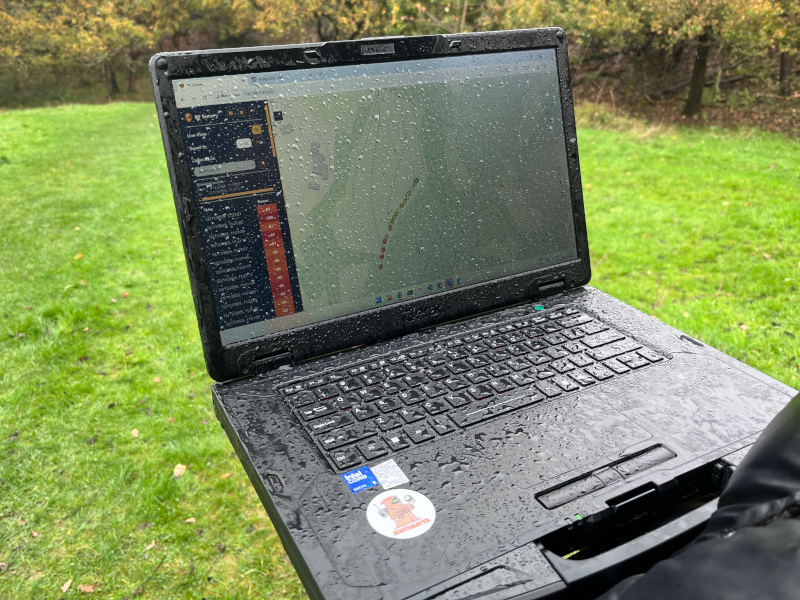
Strong LTE signals seen from a mountain

This significant variation with the possible distance is where modelling can add value to reduce the vast search area.

For the example radio, these power values in Watts must be converted to decibel milliwatts (dBm) for consistency with the path loss modelling and to establish the range in decibels which will inform simulation parameters. In this case, low power is 20dBm (0.1W) and high power is 36dBm (4W) for 16dB of uncertainty.

In an obstructed environment such as a forest, this uncertainty represents a shorter distance than in free space where again, modelling can add value. A counter drone system is an example of a free space problem.

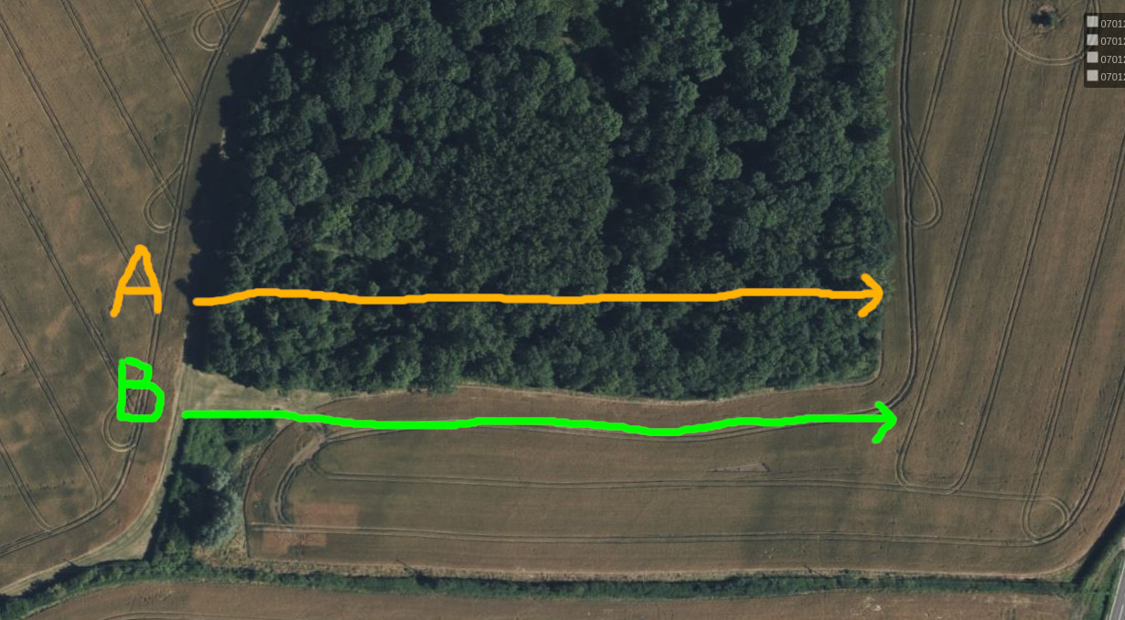
Path loss variation due to clutter attenuation

Link reciprocity

A radio link is not symmetrical due to how and where obstacles impact the fresnel zone which is the cone of power an element radiates. Even if you have line of sight (LOS) between two even power stations, you can still get different received power levels from A to B than B to A.

A to B != B to A

This matters as we cannot model the emitter since we don’t know where it is! We can only model the receiver location.

In our experience, the difference is measured in single digits and is small compared with noise which will make a bigger impact on a link’s viability. If you are operating at the edge of a system’s link budget then the reciprocal difference may be enough to make a link one way only.

For modelling a receiver we need uplink (talk-in) measurements instead of downlink (talk-out) which we normally collect for clutter and model calibration.

Field testing

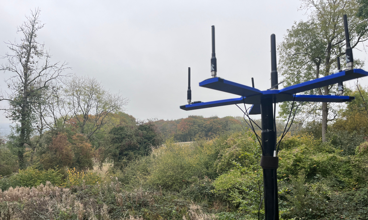
We conducted several field tests to integrate our API using a budget commercial DF receiver, the KrakenSDR. This compact entry level unit gave us a LoB (with 8 degrees of error) we could work with but as it used 8-bit SDRs, we could not rely upon the received power level as low resolution SDRs can not represent weak signals.

After a false start with a 12-bit SDR designed for the amateur community and interfaced with SoapySDR, we used a professional RFEye receiver which aside from having superior measurement accuracy and sensitivity is a turnkey solution with a web API which we have integrated with our API previously.

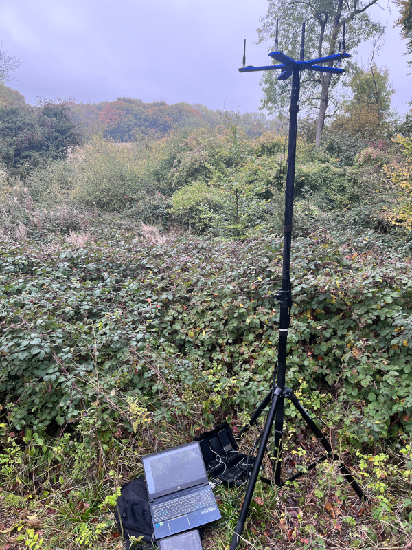
Test system

Our test system grew in scope from a Kraken with a Pi to a network in a box with a bespoke management and signal logging interface. Key to this innovation was not creating a budget DF system which we needed to collect data but the employment of an edge modelling capability on a Raspberry Pi 5.

Our goal was to develop a hardware agnostic script which our customers could use to enhance their DF data.

Hardware

  • The Line of Bearing came from a KrakenSDR with a circular 5 element array upon a 2m telescopic mast.
  • The processor was a Raspberry Pi5 running our test software and SOOTHSAYER v1.10
  • The radio traffic was generated by a Tait DMR portable radio equipped with a programming cable connected to a Pi4.
  • The power measurements came from a CRFS RFEye connected to an elevated monopole antenna.
  • A pair of sensecap meshtastic LoRa trackers were used for GPS tracking.
  • A laptop and tablet running ATAK were used to manage the system and observe the output as a KML.

Software

To automate data collection, we developed test software to collect data from the SDR and DF receiver simultaneously and model them using our API. The DMR radio was configured to broadcast telemetry periodically which provided a regular target signal and the out-of-band meshtastic tracker provided a precise location within the trees.

We couldn’t use a second DMR radio to receive the telemetry as bi-directional radio traffic risked spoiling the data.

The modelling came from SOOTHSAYER 1.10 which was installed upon the Raspberry Pi 5. This also provided the map tiles for a web based logging system which displayed live signal readings. Only one (CPU) API call was necessary per test cycle to generate a grey scale Path Loss map in decibels (dB) from which subsequent received power heat maps in decibel milliwatts (dBm) could be rapidly derived using a simple formula.

The path loss simulation needs refreshing if either the location, frequency or height change but is power agnostic. The client script queries this path loss map using known (or assumed) radio power levels.

Results are presented as a network KML which can be consumed on standards based geo-viewers like ATAK.

Challenges

We took our ‘Temu DF system’ out twice but we couldn’t collect as much data as we wanted in the time available due to different constraints such as the weather or just running a small business.

A decision to avoid vehicles and buildings was made to avoid reflections which meant we had to run the equipment from travel batteries. The power budget for the Pi5 (30W), KrakenSDR (12W) and RFEye (5W) was 47W which was more than we normally test with so it reduced our endurance.

We encountered local radio traffic on our licensed channels due to the choice of locations overlooking the city. This was easy to discount at the start of the test when our signal was obvious but became a nuisance as it faded into the trees and ultimately tainted our test data since we were triggering on power.

Old data to the rescue

After several frustrating tests where a lot of time was spent climbing local hills, calibrating DF and chasing false positives, we elected to reuse a rich data set from an antenna field test last year which included bi-directional links for a UHF radio on a moving vehicle.

This data was attractive as it included the uplink and a good variety of obstacles including houses, trees and hills as well as LOS links which are all useful for calibration. Before we could conduct DF analysis with the uplink, we calibrated the local clutter using the downlink, as we do routinely for calibration. This is a standard process we have developed a feature for in the web interface as well as a supporting video tutorial. Using our new 2m tree height data, we were able to improve upon last year’s score.

As we did not collect lines of bearings during that model test, we had to simulate these using the known vehicle location for which we used 10 degrees of azimuth error.

Somerton UHF calibration, 2024

Analysis technique

To compute the effectiveness of this technique we calculated the area of the 10 degree arc where the vehicle could have been, with a radius of 6km representing the maximum range in this test.

This gave us a search area for a given LoB of 3,141,593 m2.

Our analysis script calculated a high resolution grey scale heatmap using SOOTHSAYER’s API which was referenced with collected power readings. To compare path loss (dB) with received power (dBm) we used the known radio power of 2W (33dBm) within a link budget formula to generate received power which was compared with measurements.

RSSI (dBm) = Radio Power (dBm) + Gain (dBi) - Path Loss (dB) - Losses (dB) + Receiver Gain (dBi) - Receiver Loss (dB)

Where the difference between measurements and simulation was within tolerances of our colour key, we styled that pixel, otherwise we eliminate it from the search area and set it to transparent.

The result is an accuracy heatmap defined by a traffic light colour key. The levels we chose for our “known power” assessment were 1, 2 and 3dB. By showing 3dB of error we allow for receiver error and reduce the risk of false negatives where a matching location might be discounted.

When the radio power is known, we can produce more accurate results.

When the radio power is unknown and the hardware/signal is known, we can simulate the minimum and maximum power to generate a dynamic range for the analysis. We used a low power value of 20dBm (0.1W) and a high power value of 36dBm (4W) for a possible power range of 16dB so our “low accuracy” colour key was 14/15/16dB.

We repeated the analysis with known and unknown power levels to compare accuracy.

Results

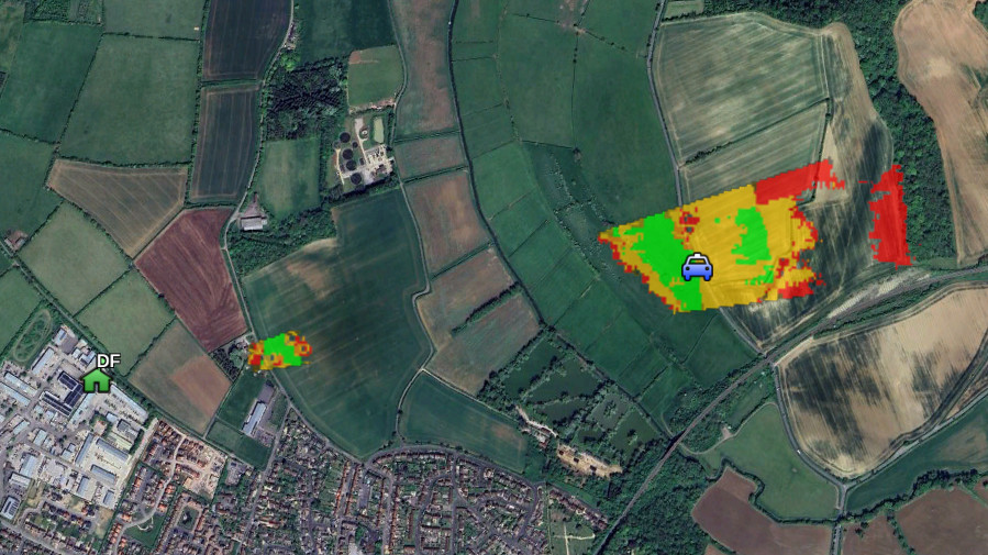
Analysis of data revealed the simulation heatmap significantly reduced the search area. As expected, knowing the radio power helps greatly but even with unknown power the search area was reduced to 32% of what it could have been for a conventional 6km arc.

Even when radio power is unknown, the search area is reduced significantly

Known Power (2W)Unknown Power (0.1 or 4W)
Best case0.010.03
Worst case27.3364.37
Average area7.93%31.51%
Improved search area as a fraction of the original arc area in m2

The amount of benefit was relative to the terrain and clutter: For example, where there were no obstacles or a single consistent obstacle such as a forest, the result was a focused band of probability without any false positives.

Where there were multiple obstacles such as a hill and a forest, false positives appeared which depending upon the ground could be discounted by an observer. This was to be expected given the pixel picking which is taking place.

A tight traffic light schema, with tuned clutter, was better than a loose schema with larger error margins. The reason being that it will show much less false positives.

Video and KMZ

This video is a sped-up compilation of time stamped KMZ layers viewed on Google Earth showing the vehicle’s route around the sensor. Where the vehicle disappears, no signal was detected.

The KMZ is available here and works best in Google Earth.

Demo video of Enhanced DF

Conclusion

This testing proved that the effectiveness of a single LoB can be improved greatly with modelling but the concept is only an improvement if the analysis is automated as doing this manually would not be faster than a map study.

The reason this analysis isn’t performed regularly by DF systems today isn’t for a lack of LoBs and RSSI measurements but rather a lack of APIs with which to exploit this information. Current RF planning software exists as a user interface which requires manual, and skilled, operation. Furthermore, the capability often exists in the wrong location on a high performance desktop computer, disconnected from edge sensors.

By putting this API at the edge on small board computers (SBCs) such as the Raspberry Pi 5 or Nvidia Jetson, a DF system’s effectiveness can be improved. Through open GIS standards like KML, the result can be consumed on open standard GIS systems like ATAK requiring minimal integration effort to add a powerful capability.

Looking forward, we are speaking with open minded vendors about adding this API to enhance existing systems.

If you’d like to improve your LoBs, get in touch with us or one of our regional resellers.

Links

SOOTHSAYER server: https://cloudrf.com/soothsayer

Kraken SDR: https://www.krakenrf.com/

DF integration demo: https://github.com/Cloud-RF/CloudRF-API-clients/tree/master/integrations/DF

API schema: https://cloudrf.com/documentation/developer

Posted on

Saving water with Radio

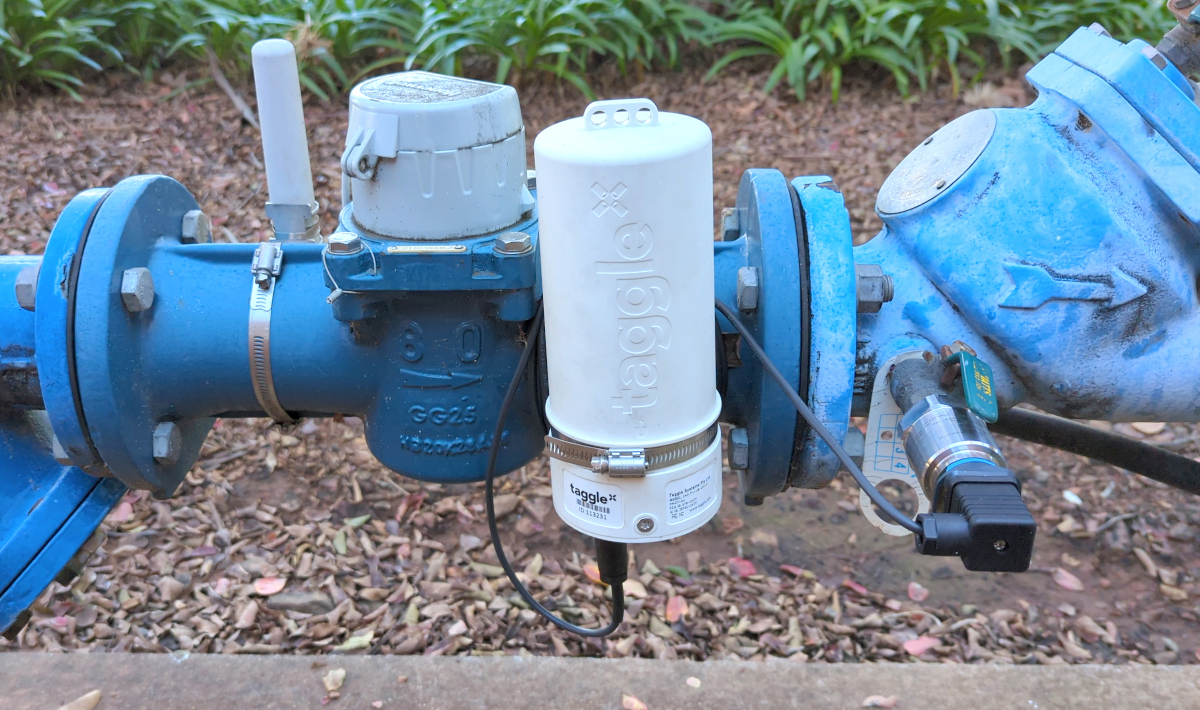
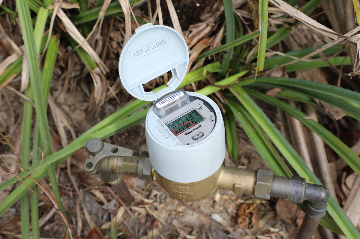
Taggle supplies the Australian water industry with innovative smart water meters and analytics, connected with Taggle’s Byron DSSS sub GHz radio technology, which is Australia’s most widely deployed LPWAN technology.

As a long time CloudRF customer, Taggle use the service to efficiently plan and deploy new gateway sites and also to monitor ongoing performance and expansion on existing sites. The ability to use CloudRF while in the field, onsite, makes it a useful tool during deployment.

Over 65 councils and water utilities across Australia use Taggle’s solutions to ensure that water, an increasingly precious commodity, is used as efficiently as possible resulting in significant cost savings and environmental benefits for customers and communities.

Posted on

Critical Coronation private 5G network planned with CloudRF

On Saturday 6th May the worlds media descended on London for the Coronation of King Charles, an event last planned before many people had television.

As the national broadcaster, the BBC managed the coverage and worked with Neutral Wireless to deploy an innovative private 5G network, with dedicated spectrum, along the procession route for exclusive use by the media and special cameras with 5G modems.

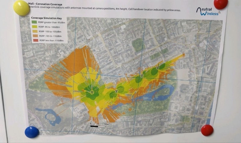
Using the CloudRF API with UK LiDAR data the team created accurate urban line of sight models for their N77 base stations along the tree lined route. Their model used RSRP units and a custom colour schema to map the 4GHz downlink coverage and key handover regions to ensure smooth subscriber transitions for the dynamic event. 

Antenna patterns

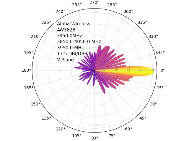
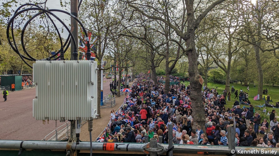
The area to be covered is a linear tree lined boulevard known as “The Mall” which leads to one of the most iconic buildings in the country, Buckingham palace. For this task, high performance Alpha Wireless directional panels were employed above the crowds at only 4m, much lower than a conventional city cellular network where a mast will be on rooftops. The combination of low height and a 4GHz frequency limits the effective range so the direction of the antennas needed to be carefully optimised to provide maximum coverage for broadcasters, strategically positioned along the route for line of sight.

How do you model a parade of horses?

Given the low height of the masts and the significant number of tall horses on parade this presents a challenge to critical line of sight which a LiDAR vendor cannot help with. The same problem applies to temporary structures such as the grandstand erected outside the Palace.

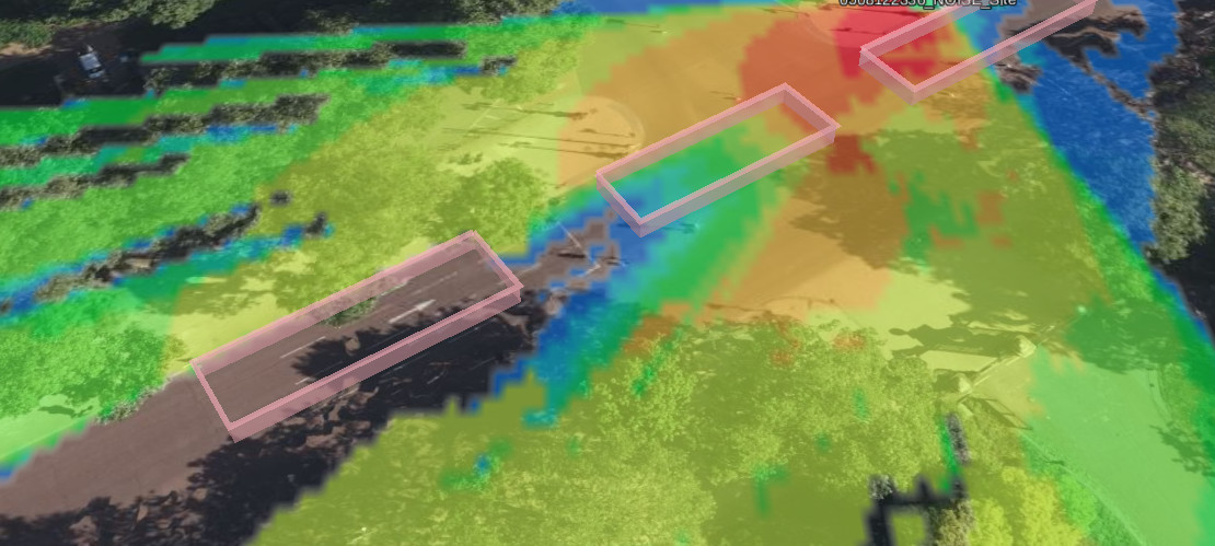
For a challenge such as this we can use custom clutter to simulate a parade of horses at a uniform distribution with a nominal density value. A “brick” clutter type can be customised to 2m height and 0.4dB/m attenuation to simulate loss through the parade to show the low and high risk locations for maintaining a link through the parade.

Our current 2D engine regards all obstacles as extending to the ground so a clutter model for a horse will be conservative since in reality a horse has a substantial gap between its legs sufficient for some RF to travel between it and reflect, and diffuse, off the rough ground to reach a camera beyond it. We’re already working on 3D 😉

In the screenshot below, the formation nearest the mast present no challenge, the formation in the middle show attenuation throughout them making a link difficult potentially depending upon siting of the receiver and the distant formation is blocking the, already attenuated, signal.

Trees

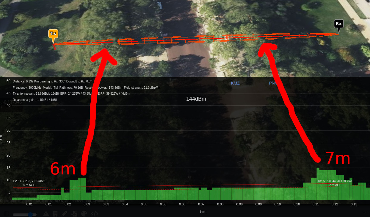
The parade was held in May when the trees along the Mall are coming into leaf presenting a moderate obstacle to the 4GHz frequencies. The temporary masts were therefore erected forward of the trees for optimal coverage but still technically under the canopy which makes planning challenging with a 2D engine since these trees can exist as spikes in the LiDAR profile. To avoid accidentally siting a mast atop a tree/spike in the model the path profile tool can be used to inspect the path profile, to identify where there are tall trees in the underlying surface model. Using the UK Environment Agency LiDAR from 2019, the nearest trees on the Mall are lightly represented in LiDAR with a 6m to 8m average canopy compared to their significant neighbours one row back and beyond in St James Park.

The result

The high resolution coverage map was integrated with official event mapping, printed, and displayed in the event broadcasting operations room as a reference. You can also see it on the BBC.

Despite the challenges expected from such congested spectrum, dynamic obstructions and the unexpected surprise of unscheduled electronic counter measures they were able to deliver accurate coverage, on time and within budget to broadcast a historic event in high definition, in real time.

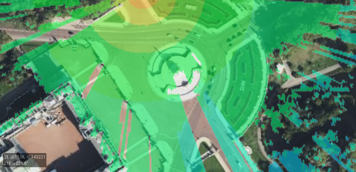
Victoria Memorial

CloudRF referenced in award winning technical paper

The BBC research and development team published an award winning paper at the 2023 International Broadcasting Convention about the event titled 5G Standalone Non-Public Networks: Modernising wireless production.

In this paper, the 4GHz coverage accuracy was validated using ground truth data. This quote about CloudRF’s accuracy stands out:

The agreement between the predictions and on-the-ground measurements is excellent

BBC Research and Development

You can download the paper at the BBC here.

Posted on

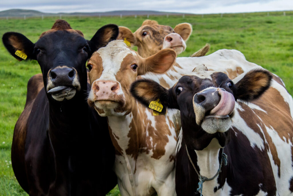
Connecting smart cows to moove data

Smart farming

Smart farming is using Internet of Things (IoT) technologies in agriculture to enable efficient use of resources.

For this blog we’re focused on cattle farming on large, fence-less farms in New Zealand. The farms in question are vast and remote so connectivity options are limited. This is why an off-grid sub-GHz LPWAN network is ideal due to its long range and the requirement to only send small, infrequent, packets of data.

For the solution to be cost-effective compared with Satellite, as little infrastructure as possible is needed which in this case is a LPWAN gateway on a pole, some collars for the herd and an app to manage the system via a web service.

Siting the LPWAN gateway(s) properly is critical to achieving not only coverage across the farm(s) but to reduce the number of gateways, which reduces complexity and cost.

Sub GHz LPWAN on the farm

An 868MHz LPWAN signal can go for many miles under the right conditions. We know this well from powering the Helium LPWAN network’s planning tool, Helium Vision, where people can communicate data 50 miles with a fraction of a watt of RF power and an omni directional antenna.

Despite it’s useful diffraction properties which enables it to work non-line-of-sight (NLOS), it’s still sensitive to obstructions so clutter on the farm such as buildings and trees needs modelling accurately. CloudRF has 10m Landcover for New Zealand from the European Space Agency and 10m DSM from the LINZ Geospatial agency.

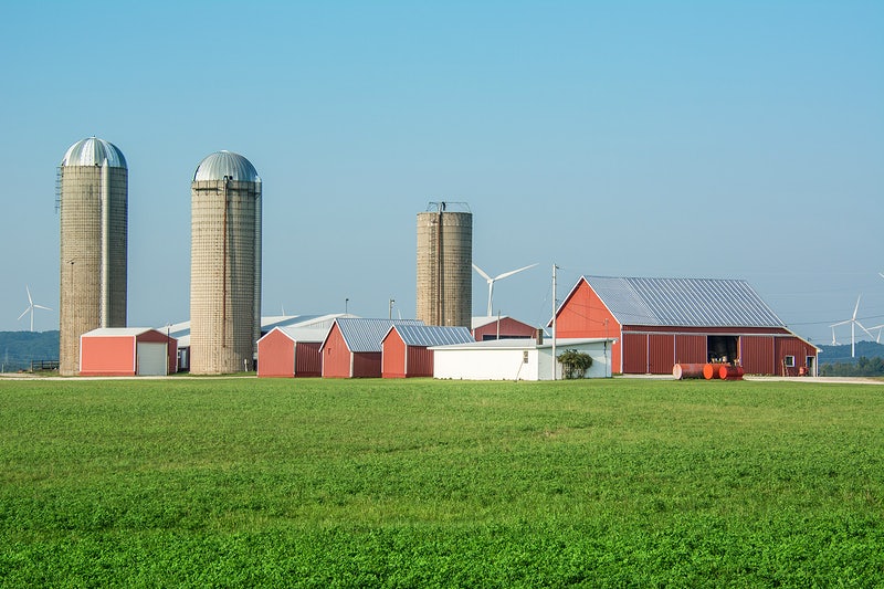
These data sets are adequate for most outdoor scenarios but are not fine enough to model a farm complex of buildings, such as tall grain silos, metal sheds and seasonal obstacles. For high resolution you could source your own surface model, as our customer Halter did…

Farm buildings and silos

Use case: Halter

Halter are a novel agri-tech startup focused on cattle management with a unique solar powered collar.

They needed accessible RF planning software to help their engineers site LPWAN gateways. Having used and liked Cloud-RF, they needed higher resolution surface models of the farms, and no pesky API restrictions!

They also planned to build their own tools on top of our powerful physics based API which is smart as it allows their R&D team to focus on their primary product, and not waste time reinventing the wheel.

Their options were either buy expensive commercial data or self generate data using a drone and photogrammetry software such as Pix4D. Given the prohibitive cost of high resolution commercial LiDAR, it would only take a few jobs to make a return on the purchase of a decent drone!

https://halterhq.com/

Halter purchased a private Keyhole Radio server from us which included the API they needed. The server runs as virtual machine and crucially, lets them import their own terrain data.

They were quickly able to import high resolution, organic data into their server as GeoTIFF files. This allowed them to work with data which was very current, even hours old, so would be an accurate model of tree heights and man made obstructions.

The terrain format accepted by Keyhole Radio and SOOTHSAYER is GeoTIFF, Int16 resolution and WGS84 (EPSG:4326) projection.

LPWAN coverage on a farm in New Zealand

1m resolution

It wasn’t all plain sailing though, they found that there was a limit to the physical tile sizes our server could use caused by memory. The solution was to reprocess the large tile into smaller tiles to make it digestible.

A 5000 x 5000 GeoTIFF at Int16 resolution will require 50MB of disk space. If this is 5m LiDAR, the physical width is 25km x 25km. Our engine can super-sample, so if you used this tile, but requested 1m resolution, it would create a raster in memory measuring 25,000 x 25,000 pixels which would need 1.25GB of memory.

For 1m resolution however, tiles measuring 1000 x 1000px would only require 2MB of disk and memory. You may need to load in a few, lets say 16, to do your model but that’s still only 32MB.

You could also resolve this by increasing the memory available to the server but it’s recommended to prepare data into smaller parcels. We support 1m resolution in our API but don’t hold a lot of 1m data sets due to their substantial cost and size. If you already have 1m data, a Keyhole Radio or SOOTHSAYER server is the answer.

1m resolution

Summary
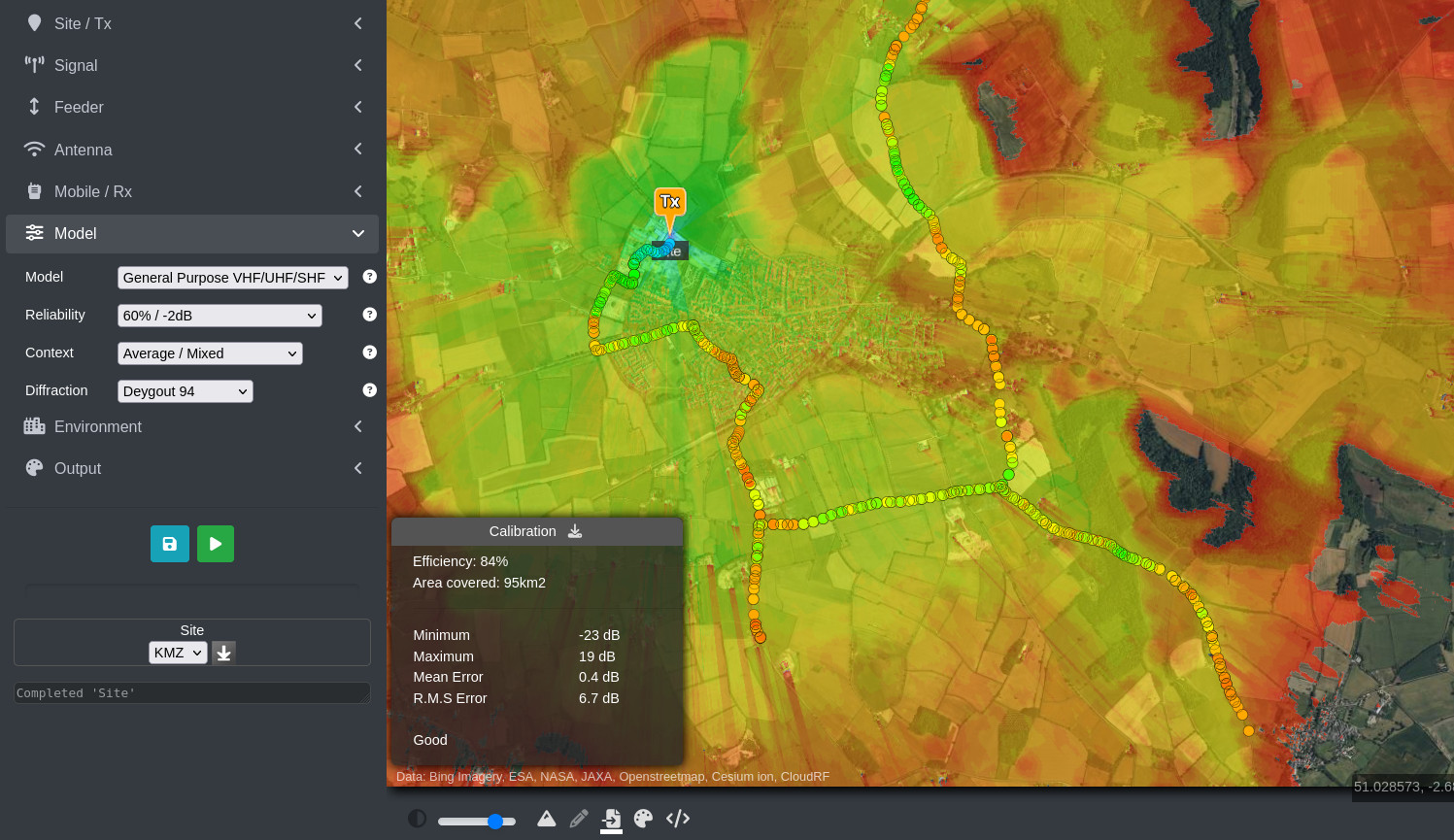
Cloud-RF’s powerful API is ideal for efficient smart farming.

Our private servers will let you take it to the next level with terrain data you can source yourself, no API restrictions and as a bonus, they work without an internet connection!
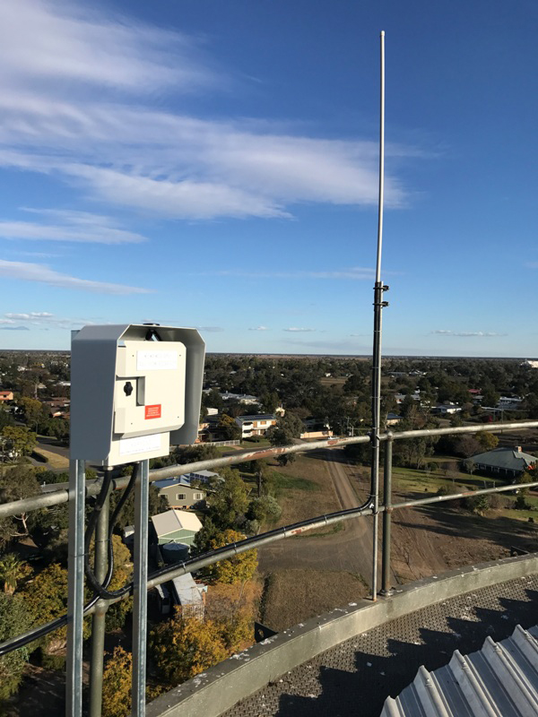
Finally, all our jokes are offal.