


API
The CloudRF API offers a powerful and scalable service to model diverse radio networks anywhere in the world at high resolution.
When integrated into another system, it can automate modelling to save significant development effort with a modest budget.
The rapid nature of its processing enables live processing for dynamic systems such as spectrum management or autonomous vehicles.
Use cases
Automate customer qualification based upon a postal address
Robot route selection
Best site analysis for optimising deployments
Receiver modelling for signal multi-lateration
Generation of network coverage maps for marketing or briefings
Automated regression testing for network changes
Integration with cognitive radios for dynamic reconfiguration
OpenAPI Schema
For a complete OpenAPI version 3 schema of the CloudRF API please consult the OpenAPI documentation.
API Endpoint
For CloudRF users, the API endpoint is https://api.cloudrf.com.
Users with a private SOOTHSAYER server will have an IP address or custom domain name instead. The API endpoints and parameters are the same and are protected with TLS encryption.
Authentication
Each user has a unique private API key which resembles a long random string of characters. You should protect this key to prevent unauthorised use of your account.
An example of an API key is as below:
101-ec94622a4cb939a77101a118c6871d03cea88af3
Using Your API Key
The CloudRF API requires API key authentication in the request header. This provides a key-value pair with key as the first value and your personal key as the second, paired value.
For example, Postman allows you to enter your key from their interface.
Key Security
It is important to keep your API key secure. Publicly exposing your key can compromise your account, which could result in a loss of data or unexpected charges. A key does not give access to your interface or account management which is separate.
To keep your API keys secure, follow some best practices:
Keys as Variables
Store API keys as environment variables. This has an added benefit of accessing your key via a friendly environment variable name rather than having to remember your full key each time.
Do not embed API keys directly in code as they will be exposed eventually.
Keys as Private Files
You can store your API key in a private file and reference that file each time you need to use your API key.
If you store API keys in files, store those files outside your application’s source tree.
Doing so helps to ensure that your keys do not end up in your source code version control system. This is particularly important if you use a public source code management system such as GitHub.
“Hello World!” Example
Send this curl request to model coverage for a UHF radio, 2m above the ground with 2W of power:
curl --location 'https://api.cloudrf.com/area' \
    --header 'key: YOUR-API-KEY-HERE' \
    --data '{
        "site": "HelloWorld",
        "network": "Testing",
        "transmitter": {
            "lat": 38.916,
            "lon": 1.448,
            "alt": 2,
            "frq": 450,
            "txw": 2,
            "bwi": 0.012
        },
        "receiver": {
            "lat": 0,
            "lon": 0,
            "alt": 2,
            "rxg": 0,
            "rxs": -105
        },
        "antenna": {
            "txg": 0,
            "txl": 0,
            "ant": 1,
            "azi": 0
        },
        "environment": {
            "clt": "Temperate.clt",
            "landcover": 1,
            "buildings": 1,
            "terrain": 2
        },
        "output": {
            "units": "metric",
            "col": "LTE.dBm",
            "out": 2,
            "res": 10,
            "rad": 5
        }
    }'
Example API Requests
Below lists some basic examples of some of the most common types of requests made to the CloudRF API.
For a complete list of available schemas please consult the OpenAPI documentation.
With all requests some values are required and so the response will return any validation errors or any failures should your request not be able to be processed.
Area
The area endpoint accepts a JSON object in the request body describing your network and will run a point-to-multipoint “heatmap” calculation.
Request
The below example is for an omni-directional antenna on an 8m mast at 446MHz. The request is sent as a POST request to https://api.cloudrf.com/area and it will return a JSON response containing metadata and URLs to image layers for your map.
{
    "site": "Harbour",
    "network": "PMR",
    "engine": "2",
    "transmitter": {
        "lat": "38.913767",
        "lon": "1.440017",
        "alt": "8",
        "frq": "446",
        "txw": "1",
        "bwi": "0.1"
    },
    "receiver": {
        "lat": 0,
        "lon": 0,
        "alt": "2",
        "rxg": "2",
        "rxs": "-90"
    },
    "antenna": {
        "txg": "2.15",
        "txl": "0",
        "ant": "1",
        "azi": "0",
        "tlt": "0",
        "fbr": "0",
        "pol": "v"
    },
    "model": {
        "pm": "1",
        "pe": "2",
        "ked": "1",
        "rel": "50"
    },
    "environment": {
        "clt": "Minimal.clt",
        "elevation": "2",
        "landcover": "1",
        "buildings": "0",
        "obstacles": "0"
    },
    "output": {
        "units": "m",
        "col": "RAINBOW45.dBm",
        "out": "2",
        "nf": "-124",
        "res": "20",
        "rad": "8"
    }
}
Response
The PNG_Mercator image is warped for slippy maps like Mapbox, Leaflet and Google Maps. The PNG_WGS84 is for globes like Google Earth, Cesium and WinTAK.
{
    "kmz": "https://api.cloudrf.com/archive/eFYyWFpUYW0zR1pxcTIyRlRKREQxUT09/kmz",
    "PNG_Mercator": "https://api.cloudrf.com/users/1/0812210016_PMR_harbour.3857.png",
    "PNG_WGS84": "https://api.cloudrf.com/users/1/0812210016_PMR_harbour.4326.png",
    "bounds": [
        39.00613,
        1.532378,
        38.82141,
        1.347656
    ],
    "id": 8191195,
    "sid": "eFYyWFpUYW0zR1pxcTIyRlRKREQxUT09",
    "area": 55.9,
    "coverage": 28.0,
    "key": [
        {
            "l": "-45dBm",
            "r": 37,
            "g": 131,
            "b": 255
        },
        {
            "l": "-55dBm",
            "r": 46,
            "g": 254,
            "b": 187
        },
        {
            "l": "-65dBm",
            "r": 98,
            "g": 254,
            "b": 55
        },
        {
            "l": "-75dBm",
            "r": 254,
            "g": 234,
            "b": 63
        },
        {
            "l": "-85dBm",
            "r": 254,
            "g": 72,
            "b": 72
        }
    ],
    "elapsed": 2297.0,
    "balance": 23476
}
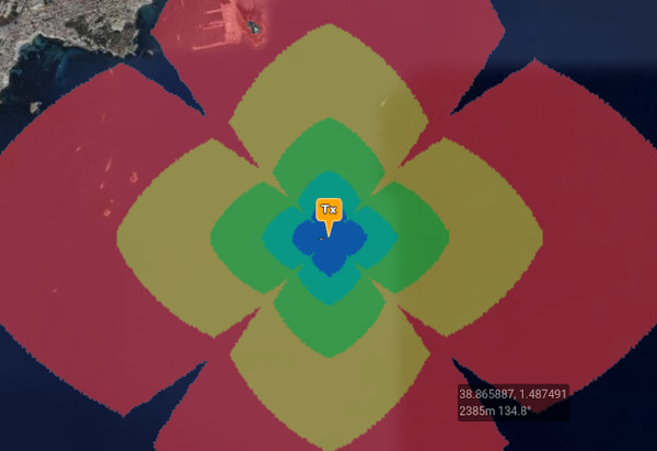
PNG image with RGB colours which map to the signal levels in the JSON output:
Go Faster with the GPU Engine
Switch the engine parameter to 1 to use the GPU engine. All other settings are the same.
{
    "site": "Harbour",
    "network": "PMR",
    "engine": "1",
    ... snipped for brevity ...
}
Please note that to be able to make use of the GPU engine you require an active GPU subscription or SOOTHSAYER with GPU functionality enabled.
Multi-Azimuth Requests
You can specify an array of azimuths to model panels on a cell tower for custom patterns and templates. Pass azimuths in as a comma separated list in quotes like "0,90,180,270". The maximum number of azimuths you can pass in one API request is 90. This works for CPU and GPU engines.
{
    "site": "FourPanels",
    "network": "800MHZ",
    "engine": "2",
    "transmitter": {
        "lat": "38.881037",
        "lon": "1.468",
        "alt": "12",
        "frq": "800",
        "txw": "1",
        "bwi": "0.1"
    },
    "receiver": {
        "lat": 0,
        "lon": 0,
        "alt": "2",
        "rxg": "2",
        "rxs": "-90"
    },
    "antenna": {
        "txg": "21",
        "txl": "0",
        "ant": 0,
        "azi": "0,90,180,270",
        "tlt": "1",
        "hbw": "80",
        "vbw": "80",
        "fbr": "21",
        "pol": "v"
    },
    "model": {
        "pm": "11",
        "pe": "2",
        "ked": "1",
        "rel": "50"
    },
    "environment": {
        "clt": "Minimal.clt",
        "elevation": "2",
        "landcover": "0",
        "buildings": "0",
        "obstacles": "0"
    },
    "output": {
        "units": "m",
        "col": "RAINBOW45.dBm",
        "out": "2",
        "nf": "-120",
        "res": "20",
        "rad": "5"
    }
}
Path
The path endpoint accepts a JSON object describing your network and will run a point-to-point calculation.
Request
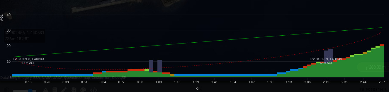
The following example includes some optional parameters and provides the required data to model a link with landcover and 3D buildings enabled at 30m resolution. The request is similar to the area call except the receiver latitude (lat) and longitude (lon) values are populated.
The below example is sent as a POST request to https://api.cloudrf.com/path.
{
    "site": "HarbourLink",
    "network": "LPWAN",
    "transmitter": {
        "lat": "38.9090",
        "lon": "1.44094",
        "alt": 12,
        "frq": "868",
        "txw": "0.1",
        "bwi": "0.1"
    },
    "receiver": {
        "lat": "38.9173881",
        "lon": "1.46864923",
        "alt": 12,
        "rxg": "2",
        "rxs": "-90"
    },
    "antenna": {
        "txg": "2.15",
        "txl": "0",
        "ant": "1",
        "azi": "0",
        "tlt": "0",
        "pol": "v"
    },
    "model": {
        "pm": "1",
        "pe": "2",
        "ked": "1",
        "rel": "95"
    },
    "environment": {
        "clt": "Minimal.clt",
        "elevation": "2",
        "landcover": "1",
        "buildings": "1",
        "obstacles": "0"
    },
    "output": {
        "units": "m",
        "col": "RAINBOW45.dBm",
        "out": "2",
        "res": "30",
        "rad": "2"
    }
}
Response
The response contains metadata about the link along with raw values necessary to build a chart using a graphing library such as Matplotlib or Plotly. It also contains a link to a KMZ so you can see the profile in 3D.
{
    "Engine": "Sleipnir 1.7.8",
    "Frequency MHz": 868,
    "Propagation model": "ITM",
    "Earth dielectric constant": 13,
    "Earth conductivity": 0.002,
    "Radio climate": "Maritime Temperate (Land)",
    "Atmospheric bending constant": 301,
    "Fraction of situations": 95,
    "Fraction of time": 95,
    "Receiver": [
        {
            "Latitude": 38.91739,
            "Longitude": 1.468649,
            "Ground elevation m": 28,
            "Antenna height m": 12,
            "Receiver gain dBd": -0.15,
            "Receiver gain dBi": 2
        }
    ],
    "Transmitters": [
        {
            "Latitude": 38.90908,
            "Longitude": 1.440943,
            "Ground elevation m": 1,
            "Antenna height m": 12,
            "Distance to receiver km": 2.572,
            "Azimuth to receiver deg": 68.92,
            "Downtilt angle deg": 0.6,
            "Antenna gain dBd": 0,
            "Antenna gain dBi": 2.15,
            "Polarisation": "Vertical",
            "Power W": 0.1,
            "Power dBm": 22.15,
            "ERP W": 0.1,
            "EIRP W": 0.164,
            "ERP dBm": 20,
            "EIRP dBm": 22.15,
            "Free space path loss dB": 95.3,
            "Bandwidth MHz": 0.1,
            "Johnson Nyquist noise dB": 0.2,
            "Noise floor dBm": -120,
            "Channel noise dBm": -119.8,
            "Signal power at receiver dBm": -88.6,
            "Signal to Noise Ratio dB": 31.2,
            "Computed path loss dB": 108.6,
            "Model attenuation dB": 13.3,
            "Field strength at receiver dBuV/m": 49.6,
            "RX voltage 50 ohm dipole uV": 14,
            "RX voltage 50 ohm dipole dBuV": 23,
            "RX voltage 75 ohm dipole uV": 17,
            "RX voltage 75 ohm dipole dBuV": 24,
            "Raise RX antenna for LOS": 0,
            "Raise RX antenna for fresnel 60%": 0,
            "Raise RX antenna for full fresnel": 19,
            "Obstructions": [],
            "Distance": [
                0.03,
                0.059,
                0.089,
                0.119,
                0.148,
                ... snipped for brevity ...
            ],
            "Terrain": [
                1,
                1,
                1,
                1,
                1,
                ... snipped for brevity ...
            ],
            "Terrain_AMSL": [
                1,
                0,
                0,
                0,
                0,
                ... snipped for brevity ...
            ],
            "Landcover distance": [
                0.03,
                0.059,
                0.089,
                0.119,
                0.148,
                ... snipped for brevity ...
            ],
            "Landcover codes": [
                1,
                1,
                1,
                1,
                1,
                ... snipped for brevity ...
            ],
            "Landcover heights": [
                1,
                1,
                1,
                1,
                1,
                ... snipped for brevity ...
            ],
            "Fresnel": [
                0,
                -3.18,
                -4.47,
                -5.45,
                -6.25,
                ... snipped for brevity ...
            ],
            "dBm": [
                -50,
                -56,
                -60,
                -62,
                -64,
                ... snipped for brevity ...
            ],
            "dB": [
                70,
                76,
                80,
                82,
                84,
                ... snipped for brevity ...
            ]
        }
    ],
    "calculation_adjusted": [],
    "elapsed": 130.0,
    "Chart image": "https://api.cloudrf.com/API/archive/data?sid=c2ZrYXdUa0tPeGFrbG5wS1dLd3RIdz09&type=ppa",
    "kmz": "https://api.cloudrf.com/API/archive/data?sid=c2ZrYXdUa0tPeGFrbG5wS1dLd3RIdz09&type=path"
}
The landcover code meanings are as follows:
1Water2Trees3Grassland4Swamp5Crops6Shrubland7Built-up8Bare ground9Snow / Ice10Buildings11Custom Clutter 112Custom Clutter 213Custom Clutter 314Custom Clutter 415Custom Clutter 516Custom Clutter 617Custom Clutter 718Custom Clutter 819Custom Clutter 9
Points
The points endpoint accepts a JSON object describing an array of points (transmitters) which will be tested back to a single point (receiver).
Request
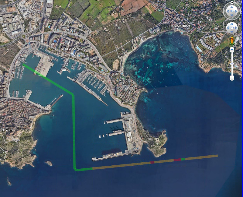
The following example is for route a boat will take. The location varies with each point but all the other values are constant.
The request is sent as a POST body to https://api.cloudrf.com/points.
{
    "site": "RIB",
    "network": "VHF",
    "transmitter": {
        "lat": 38.914381,
        "lon": 1.436988,
        "alt": "2",
        "frq": "160",
        "txw": "1",
        "bwi": "0.1"
    },
    "points": [
        {
            "lat": 38.91086406303705,
            "lon": 1.444486542453175,
            "alt": 2
        },
        {
            "lat": 38.91041372754393,
            "lon": 1.444495874752767,
            "alt": 2
        },
        {
            "lat": 38.90996339201471,
            "lon": 1.4445052069344337,
            "alt": 2
        },
        {
            "lat": 38.909513056449505,
            "lon": 1.444514538998178,
            "alt": 2
        }
    ],
    "receiver": {
        "lat": 38.914381,
        "lon": 1.436988,
        "alt": 2,
        "rxg": "2",
        "rxs": "-90"
    },
    "antenna": {
        "txg": "2.15",
        "txl": "0",
        "ant": "1",
        "azi": "0",
        "tlt": "0",
        "fbr": "2.15",
        "pol": "v"
    },
    "model": {
        "pm": "11",
        "pe": "2",
        "ked": "1",
        "rel": "50"
    },
    "environment": {
        "elevation": "2",
        "landcover": "1",
        "buildings": "0",
        "obstacles": "0"
    },
    "output": {
        "units": "m",
        "col": "RAINBOW45.dBm",
        "out": "2",
        "nf": "-124",
        "res": "30",
        "rad": "8"
    }
}
Response
The response contains JSON metadata for the points, in this case received power levels for each point.
{
    "Engine": "Sleipnir 1.7.8",
    "Frequency MHz": 160,
    "Propagation model": "Egli VHF/UHF",
    "Model subtype": "Suburban",
    "Receiver": [
        {
            "Latitude": 38.91438,
            "Longitude": 1.436988,
            "Ground elevation m": 1,
            "Antenna height m": 2,
            "Receiver gain dBd": -0.15,
            "Receiver gain dBi": 2
        }
    ],
    "Transmitters": [
        {
            "Latitude": 38.91086,
            "Longitude": 1.444487,
            "Ground elevation m": 0,
            "Antenna height m": 2,
            "Distance to receiver km": 0.758,
            "Azimuth to receiver deg": 301.08,
            "Downtilt angle deg": 0.1,
            "Antenna gain dBd": 0,
            "Antenna gain dBi": 2.15,
            "Polarisation": "Vertical",
            "Power W": 1,
            "Power dBm": 2.15,
            "ERP W": 0.001,
            "EIRP W": 1.641,
            "ERP dBm": 0,
            "EIRP dBm": 2.15,
            "Free space path loss dB": 70,
            "Bandwidth MHz": 0.1,
            "Johnson Nyquist noise dB": 0.2,
            "Noise floor dBm": -124,
            "Channel noise dBm": -123.8,
            "Signal power at receiver dBm": -66.2,
            "Signal to Noise Ratio dB": 57.6,
            "Computed path loss dB": 96.2,
            "Model attenuation dB": 26.2,
            "Field strength at receiver dBuV/m": 27.3,
            "Raise RX antenna for LOS": 5,
            "Raise RX antenna for fresnel 60%": 77,
            "Raise RX antenna for full fresnel": 128,
            "server": 1
        },
        {
            "Latitude": 38.91041,
            "Longitude": 1.444496,
            "Ground elevation m": 0,
            "Antenna height m": 2,
            "Distance to receiver km": 0.786,
            "Azimuth to receiver deg": 304.18,
            "Downtilt angle deg": 0.1,
            "Antenna gain dBd": 0,
            "Antenna gain dBi": 2.15,
            "Polarisation": "Vertical",
            "Power W": 1,
            "Power dBm": 2.15,
            "ERP W": 0.001,
            "EIRP W": 1.641,
            "ERP dBm": 0,
            "EIRP dBm": 2.15,
            "Free space path loss dB": 70.3,
            "Bandwidth MHz": 0.1,
            "Johnson Nyquist noise dB": 0.2,
            "Noise floor dBm": -124,
            "Channel noise dBm": -123.8,
            "Signal power at receiver dBm": -66.8,
            "Signal to Noise Ratio dB": 57,
            "Computed path loss dB": 96.8,
            "Model attenuation dB": 26.5,
            "Field strength at receiver dBuV/m": 26.7,
            "Raise RX antenna for LOS": 5,
            "Raise RX antenna for fresnel 60%": 80,
            "Raise RX antenna for full fresnel": 132,
            "server": 2
        },
        {
            "Latitude": 38.90996,
            "Longitude": 1.444505,
            "Ground elevation m": 0,
            "Antenna height m": 2,
            "Distance to receiver km": 0.816,
            "Azimuth to receiver deg": 307.06,
            "Downtilt angle deg": 0.1,
            "Antenna gain dBd": 0,
            "Antenna gain dBi": 2.15,
            "Polarisation": "Vertical",
            "Power W": 1,
            "Power dBm": 2.15,
            "ERP W": 0.001,
            "EIRP W": 1.641,
            "ERP dBm": 0,
            "EIRP dBm": 2.15,
            "Free space path loss dB": 70.6,
            "Bandwidth MHz": 0.1,
            "Johnson Nyquist noise dB": 0.2,
            "Noise floor dBm": -124,
            "Channel noise dBm": -123.8,
            "Signal power at receiver dBm": -67.5,
            "Signal to Noise Ratio dB": 56.3,
            "Computed path loss dB": 97.5,
            "Model attenuation dB": 26.9,
            "Field strength at receiver dBuV/m": 26,
            "Raise RX antenna for LOS": 4,
            "Raise RX antenna for fresnel 60%": 82,
            "Raise RX antenna for full fresnel": 136,
            "server": 3
        },
        {
            "Latitude": 38.90951,
            "Longitude": 1.444515,
            "Ground elevation m": 0,
            "Antenna height m": 2,
            "Distance to receiver km": 0.848,
            "Azimuth to receiver deg": 309.74,
            "Downtilt angle deg": 0.1,
            "Antenna gain dBd": 0,
            "Antenna gain dBi": 2.15,
            "Polarisation": "Vertical",
            "Power W": 1,
            "Power dBm": 2.15,
            "ERP W": 0.001,
            "EIRP W": 1.641,
            "ERP dBm": 0,
            "EIRP dBm": 2.15,
            "Free space path loss dB": 70.9,
            "Bandwidth MHz": 0.1,
            "Johnson Nyquist noise dB": 0.2,
            "Noise floor dBm": -124,
            "Channel noise dBm": -123.8,
            "Signal power at receiver dBm": -68.1,
            "Signal to Noise Ratio dB": 55.7,
            "Computed path loss dB": 98.1,
            "Model attenuation dB": 27.2,
            "Field strength at receiver dBuV/m": 25.3,
            "Raise RX antenna for LOS": 4,
            "Raise RX antenna for fresnel 60%": 85,
            "Raise RX antenna for full fresnel": 141,
            "server": 4
        }
    ],
    "calculation_adjusted": [],
    "elapsed": 111.0,
    "kmz": "https://api.cloudrf.com/API/archive/data?points=0812220045_mymesh_PPA_POINTS&uid=1",
    "json": "https://api.cloudrf.com/users/1/0812220045_mymesh_PPA_POINTS.json"
}
Best Site Analysis
The bsa endpoint accepts a JSON object in the request body describing a location with a radius, similar to an ‘area’ call except it uses a random Monte-Carlo technique to rank locations within the area to identify the best. The colour key is irrelevant for the API since the response is always a greyscale image which you must style.
Request
The below example is for a planned Sub GHz LPWAN gateway in the hills. The request is sent as a POST request to https://api.cloudrf.com/bsa and it will return a JSON response containing metadata and URLs to image layers for your map.
{
    "site": "BestSite",
    "network": "Ibiza",
    "engine": "1",
    "transmitter": {
        "lat": 38.938092,
        "lon": 1.389430,
        "alt": "2",
        "frq": "446",
        "txw": "1",
        "bwi": "0.1"
    },
    "receiver": {
        "lat": 0,
        "lon": 0,
        "alt": "2",
        "rxg": "2",
        "rxs": "-90"
    },
    "antenna": {
        "txg": "2.15",
        "txl": "0",
        "ant": "1",
        "azi": "0",
        "tlt": "0",
        "fbr": "2.15",
        "pol": "v"
    },
    "model": {
        "pm": "7",
        "pe": "2",
        "ked": "0",
        "rel": "95"
    },
    "environment": {
        "clt": "Minimal.clt",
        "elevation": "2",
        "landcover": "0",
        "buildings": "0",
        "obstacles": "0"
    },
    "output": {
        "units": "m",
        "col": "BSA8.bsa",
        "out": "7",
        "nf": "-120",
        "res": "10",
        "rad": 3
    }
}
Response
The PNG_Mercator image is warped for slippy maps like Mapbox, Leaflet and Google Maps. The PNG_WGS84 is for globes like Google Earth, Cesium and WinTAK.
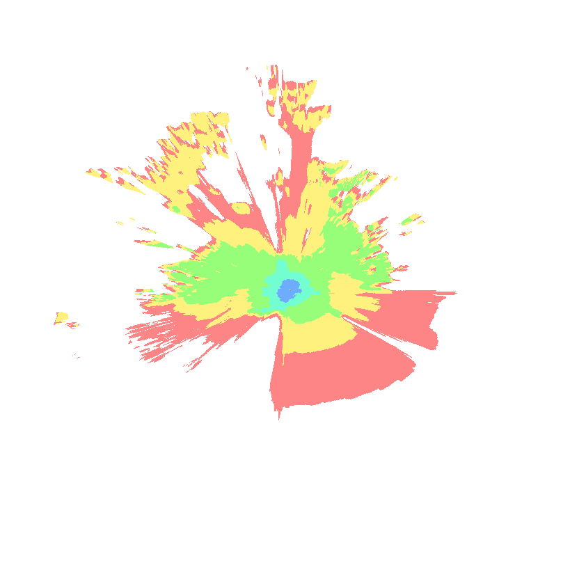
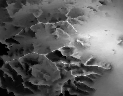
A BSA response is almost identical to an area response. The real difference is in the image which is always greyscale where white is 100% efficiency and black is 0% efficiency. The colour key returned can be used for styling by isolating only the red channel since the green and blue channels will be the same eg. RGB(254,254,254) = 95% coverage. The area and coverage fields are zero since this is not a site.
{
    "kmz": "https://api.cloudrf.com/archive/a2s1bWJkTDJYdGMrNUNHZVhpTUtUQT09/kmz",
    "PNG_Mercator": "https://api.cloudrf.com/output/projection/3857/1/0816125807_IBIZA_BestSite",
    "PNG_WGS84": "https://api.cloudrf.com/users/1/0816125807_IBIZA_BestSite.4326.png",
    "bounds": [
        38.96563941396777,
        1.4248893862148355,
        38.91054585887422,
        1.3539723152977645
    ],
    "id": 8201477,
    "sid": "a2s1bWJkTDJYdGMrNUNHZVhpTUtUQT09",
    "area": 0,
    "coverage": 0,
    "key": [
        {
            "l": "95%",
            "r": 254,
            "g": 0,
            "b": 0
        },
        {
            "l": "90%",
            "r": 254,
            "g": 91,
            "b": 0
        },
        {
            "l": "85%",
            "r": 254,
            "g": 183,
            "b": 0
        },
        {
            "l": "80%",
            "r": 236,
            "g": 254,
            "b": 0
        },
        {
            "l": "75%",
            "r": 145,
            "g": 254,
            "b": 0
        },
        {
            "l": "70%",
            "r": 53,
            "g": 254,
            "b": 0
        },
        {
            "l": "65%",
            "r": 0,
            "g": 254,
            "b": 38
        },
        {
            "l": "60%",
            "r": 0,
            "g": 254,
            "b": 129
        },
        {
            "l": "55%",
            "r": 0,
            "g": 254,
            "b": 221
        },
        {
            "l": "50%",
            "r": 0,
            "g": 198,
            "b": 255
        }
    ],
    "elapsed": 1147.0,
    "balance": 23305
}
A BSA response is shown below. Notice that ridgelines rank high, but not as high as the low ground to the east which has the best visibility of the entire area:
Request with a Polygon
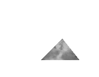
If you want to use a polygon shape to define boundaries, you can use the edges array to define each point. A minimum of 3 points are needed as lat/lon pairs within the edges array. With this you can draw political or property boundaries. A radius is automatically computed using this method so it doesn’t matter what radius you request.
{
    "edges": [
        {
            "lat": 38.94,
            "lon": 1.39
        },
        {
            "lat": 38.94,
            "lon": 1.399
        },
        {
            "lat": 38.945,
            "lon": 1.395
        }
    ],
    "site": "Triangle",
    "network": "Ibiza",
    "engine": "1",
    "transmitter": {
        "lat": 38.945,
        "lon": 1.392,
        "alt": "2",
        "frq": "446",
        "txw": "1",
        "bwi": "0.1"
    },
    ... snipped for brevity ...
}
By defining 3 points, we have reduced the study area to a triangle:
Multisite
The multisite endpoint is a GPU only function for simulating many transmitters at once. It accepts a JSON object in the request body describing an array of transmitters, using familiar fields from an area call. An antenna is defined for every transmitter so you can have different patterns in a network. You can even model a group of distant radios with omni antennas and a long range parabolic in the same request.
It renders the legacy mesh API call obsolete (unless you only have a CPU) as it merges sites by design.
Transmitters must be within 2000km of each other. eg. You cannot request a multisite across the Ocean.
Antenna azimuths must be between 0 and 359 degrees.
Request
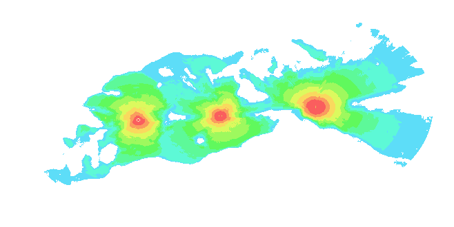
The below example is for three local UHF radios, with omni dipoles (ant: 1) in the hills. The request is sent as a POST request to https://api.cloudrf.com/multisite and it will return a JSON response containing metadata and URLs to image layers for your map.
{
    "site": "3amigos",
    "network": "UHF",
    "transmitters": [
        {
            "lat": 38.941501808741165,
            "lon": 1.3709467181497763,
            "alt": 2,
            "frq": 868,
            "txw": 1,
            "bwi": 0.1,
            "ant": 0,
            "antenna": {
                "txg": 2.15,
                "txl": 0,
                "ant": 1,
                "azi": 0,
                "tlt": 0,
                "fbr": 2.15,
                "pol": "v"
            }
        },
        {
            "lat": 38.94210625018613,
            "lon": 1.3847431304250852,
            "alt": 2,
            "frq": 868,
            "txw": 1,
            "bwi": 0.1,
            "ant": 0,
            "antenna": {
                "txg": 2.15,
                "txl": 0,
                "ant": 1,
                "azi": 0,
                "tlt": 0,
                "fbr": 2.15,
                "pol": "v"
            }
        },
        {
            "lat": 38.94370157813472,
            "lon": 1.4006969012717958,
            "alt": 2,
            "frq": 868,
            "txw": 1,
            "bwi": 0.1,
            "ant": 0,
            "antenna": {
                "txg": 2.15,
                "txl": 0,
                "ant": 1,
                "azi": 0,
                "tlt": 0,
                "fbr": 2.15,
                "pol": "v"
            }
        }
    ],
    "receiver": {
        "alt": 2,
        "rxg": 2,
        "rxs": -105
    },
    "model": {
        "pm": 11,
        "pe": 2,
        "ked": 1,
        "rel": 95
    },
    "environment": {
        "clm": 0,
        "cll": 1,
        "clt": "Minimal.clt"
    },
    "output": {
        "units": "m",
        "col": "LTE.dBm",
        "out": 2,
        "nf": -120,
        "res": 10,
        "rad": 2
    }
}
Response
The PNG_Mercator image is warped for slippy maps like Mapbox, Leaflet and Google Maps. The PNG_WGS84 is for globes like Google Earth, Cesium and WinTAK.
{
    "kmz": "https://api.cloudrf.com/archive/WUMya3l4a3ZmcVFDajZ4THZVckVuQT09/kmz",
    "PNG_Mercator": "https://api.cloudrf.com/output/projection/3857/1/0816124833_UAS_PPA_MULTISITE",
    "PNG_WGS84": "https://api.cloudrf.com/users/1/0816124833_UAS_PPA_MULTISITE.4326.png",
    "bounds": [
        38.96165650015791,
        1.4238207375342375,
        38.92354146204287,
        1.3478216615351617
    ],
    "id": 8201557,
    "sid": "WUMya3l4a3ZmcVFDajZ4THZVckVuQT09",
    "area": 43,
    "coverage": 0,
    "key": [
        {
            "l": "-60dBm",
            "r": 248,
            "g": 14,
            "b": 14
        },
        {
            "l": "-65dBm",
            "r": 248,
            "g": 107,
            "b": 14
        },
        {
            "l": "-70dBm",
            "r": 247,
            "g": 199,
            "b": 14
        },
        {
            "l": "-75dBm",
            "r": 203,
            "g": 247,
            "b": 14
        },
        {
            "l": "-80dBm",
            "r": 110,
            "g": 247,
            "b": 14
        },
        {
            "l": "-85dBm",
            "r": 17,
            "g": 246,
            "b": 13
        },
        {
            "l": "-90dBm",
            "r": 13,
            "g": 246,
            "b": 102
        },
        {
            "l": "-95dBm",
            "r": 13,
            "g": 246,
            "b": 194
        },
        {
            "l": "-100dBm",
            "r": 13,
            "g": 205,
            "b": 245
        },
        {
            "l": "-105dBm",
            "r": 13,
            "g": 113,
            "b": 245
        }
    ],
    "elapsed": 430.0,
    "balance": 23248
}
RADAR with Mixed Heights Example
The below example shows how to use the multisite API with RADAR transmitters (model.pm value of 8) where the transmitters are positioned with an elevation relative to the ground (AGL), and the receiver has an elevation above sea level (AMSL). This is indicated with an output.tx_units value of m and output.rx_units value of m_amsl, respectively.
{
    "site": "Multisite",
    "network": "RADAR_TEST",
    "transmitters": [
        {
            "lat": 30.510523,
            "lon": -86.830194,
            "alt": 5,
            "frq": 8000,
            "txw": 100,
            "bwi": 1.2,
            "antenna": {
                "txg": 15,
                "txl": 0,
                "ant": 1,
                "azi": 0,
                "tlt": 0,
                "fbr": 0,
                "pol": "v"
            }
        },
        {
            "lat": 30.500163,
            "lon": -86.814786,
            "alt": 5,
            "frq": 8000,
            "txw": 100,
            "bwi": 1.2,
            "antenna": {
                "txg": 15,
                "txl": 0,
                "ant": 1,
                "azi": 0,
                "tlt": 0,
                "fbr": 0,
                "pol": "v"
            }
        }
    ],
    "receiver": {
        "alt": 500,
        "rxg": 0,
        "rxs": -100
    },
    "model": {
        "pm": 8,
        "pe": 2,
        "ked": 1,
        "rel": 50,
        "rcs": 100
    },
    "environment": {
        "elevation": 2,
        "cll": 0,
        "clm": 0,
        "clt": "Minimal.clt"
    },
    "output": {
        "tx_units": "m",
        "rx_units": "m_amsl",
        "col": "RAINBOW.dBm",
        "out": 2,
        "nf": -120,
        "res": 50,
        "rad": 100
    }
}
Merge
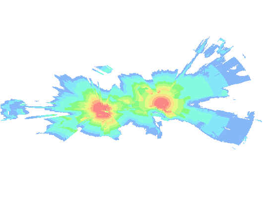
The merge function, previously mesh, is a legacy function which merges pre-calculated layers into a composite layer. This function is now done automatically with the multisite function but this is still useful for post-processing such as creating network coverage maps.
Request
The below example is a HTTP GET request for meshing the layers (max 1000) belonging to the BLUENET network and using the name mymap for the output. You must send your API key in the request header as normal.
https://api.cloudrf.com/mesh?network=BLUENET&name=mymap
You can also specify up to 100 sites in the URL as a list:
https://api.cloudrf.com/mesh?network=mymap&calcs=0816143545_BLUENET_Site,0816143541_BLUENET_Site
Response
The response is a JSON object containing images and metadata about the calculations which were used to create the mesh image:
{
    "kmz": "https://api.cloudrf.com/archive/WkYveUVDdmZTNG1IbDdPbjVKUVVLUT09/kmz",
    "PNG_Mercator": "https://api.cloudrf.com/output/projection/3857/1/0816133557_Mesh",
    "PNG_WGS84": "https://api.cloudrf.com/users/1/0816133557_Mesh.4326.png",
    "bounds": [
        51.99334,
        -2.159573,
        51.76476,
        -2.378462
    ],
    "id": 3541,
    "sid": "WkYveUVDdmZTNG1IbDdPbjVKUVVLUT09",
    "key": [
        {
            "l": "50dB",
            "r": 115,
            "g": 242,
            "b": 15
        },
        {
            "l": "45dB",
            "r": 150,
            "g": 243,
            "b": 14
        },
        {
            "l": "40dB",
            "r": 186,
            "g": 243,
            "b": 12
        },
        {
            "l": "35dB",
            "r": 222,
            "g": 243,
            "b": 11
        },
        {
            "l": "30dB",
            "r": 243,
            "g": 228,
            "b": 11
        },
        {
            "l": "25dB",
            "r": 243,
            "g": 192,
            "b": 10
        },
        {
            "l": "20dB",
            "r": 243,
            "g": 155,
            "b": 9
        },
        {
            "l": "15dB",
            "r": 243,
            "g": 118,
            "b": 9
        },
        {
            "l": "10dB",
            "r": 242,
            "g": 81,
            "b": 8
        },
        {
            "l": "5dB",
            "r": 242,
            "g": 44,
            "b": 8
        },
        {
            "l": "0dB",
            "r": 242,
            "g": 7,
            "b": 7
        }
    ],
    "elapsed": 697.0,
    "balance": 10000000000,
    "resolution": 5
}
Interference
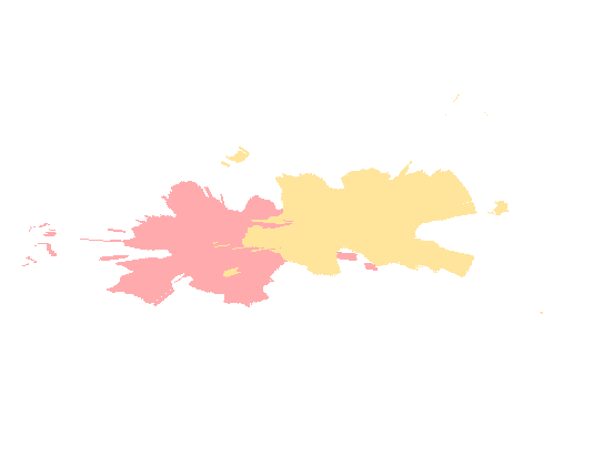
The interference function compares a set pre-calculated ‘signal’ sites with a set of pre-calculated ‘noise’ sites, and calculates a Jamming-to-Signal ratio per pixel.
Signal sites can be specified with either a network name s_network or an array of site names s_sites, interferers are specified similarly with j_network and j_sites.
Request
The below example is a HTTP POST request for comparing the layers (max 1000) belonging to the InterferenceSignal network against three specified layers from the InterferenceJamming network. The name QRM2 is used for the output, and the JS.dB colour scheme is specified. You must send your API key in the request header as normal.
{
    "s_network": "InterferenceSignal",
    "j_sites": [
        "1125164804_InterferenceJamming_A",
        "1125164820_InterferenceJamming_B",
        "1125164852_InterferenceJamming_D"
    ],
    "name": "InterferenceExample",
    "colour_key": "JS.dB"
}
Response
The response is a JSON object containing images and metadata about the calculations which were used to create the interference image:
{
    "kmz": "https://localhost/archive/M3paazRnWE84Nk0xWWc2d2RzT05zZz09/kmz",
    "PNG_Mercator": "https://localhost/output/projection/3857/1/1126160715_InterferenceExample_QRM",
    "PNG_WGS84": "https://localhost/users/1/1126160715_InterferencExample_QRM.4326.png",
    "bounds": [
        51.99334,
        -2.159573,
        51.76476,
        -2.378462
    ],
    "id": 3541,
    "sid": "M3paazRnWE84TG4xWWc2d2RzT05zZz09",
    "key": [
        {
            "l": "12dB",
            "r": 254,
            "g": 0,
            "b": 0
        },
        {
            "l": "11dB",
            "r": 254,
            "g": 21,
            "b": 0
        },
        {
            "l": "10dB",
            "r": 254,
            "g": 43,
            "b": 0
        },
        {
            "l": "9dB",
            "r": 254,
            "g": 64,
            "b": 0
        },
        {
            "l": "8dB",
            "r": 254,
            "g": 85,
            "b": 0
        },
        {
            "l": "7dB",
            "r": 254,
            "g": 106,
            "b": 0
        },
        {
            "l": "6dB",
            "r": 254,
            "g": 128,
            "b": 0
        },
        {
            "l": "5dB",
            "r": 254,
            "g": 149,
            "b": 0
        },
        {
            "l": "4dB",
            "r": 254,
            "g": 170,
            "b": 0
        },
        {
            "l": "3dB",
            "r": 254,
            "g": 191,
            "b": 0
        },
        {
            "l": "2dB",
            "r": 254,
            "g": 212,
            "b": 0
        },
        {
            "l": "1dB",
            "r": 254,
            "g": 234,
            "b": 0
        },
        {
            "l": "0dB",
            "r": 254,
            "g": 254,
            "b": 0
        },
        {
            "l": "-1dB",
            "r": 234,
            "g": 254,
            "b": 0
        },
        {
            "l": "-2dB",
            "r": 213,
            "g": 254,
            "b": 0
        },
        {
            "l": "-3dB",
            "r": 191,
            "g": 254,
            "b": 0
        },
        {
            "l": "-4dB",
            "r": 170,
            "g": 254,
            "b": 0
        },
        {
            "l": "-5dB",
            "r": 149,
            "g": 254,
            "b": 0
        },
        {
            "l": "-6dB",
            "r": 128,
            "g": 254,
            "b": 0
        },
        {
            "l": "-7dB",
            "r": 106,
            "g": 254,
            "b": 0
        },
        {
            "l": "-8dB",
            "r": 85,
            "g": 254,
            "b": 0
        },
        {
            "l": "-9dB",
            "r": 64,
            "g": 254,
            "b": 0
        },
        {
            "l": "-10dB",
            "r": 43,
            "g": 254,
            "b": 0
        },
        {
            "l": "-11dB",
            "r": 21,
            "g": 254,
            "b": 0
        },
        {
            "l": "-12dB",
            "r": 0,
            "g": 254,
            "b": 0
        }
    ],
    "elapsed": 810.0,
    "balance": 10000000000,
    "resolution": 10,
    "percentages_above_js": [
        {
            "js": 12.0,
            "percentage": 11.737680295098624
        },
        {
            "js": 9.0,
            "percentage": 21.294148830428732
        },
        {
            "js": 6.0,
            "percentage": 32.65301614648908
        },
        {
            "js": 3.0,
            "percentage": 45.59119121772359
        },
        {
            "js": 0.0,
            "percentage": 59.5531553022773
        },
        {
            "js": -3.0,
            "percentage": 71.56362511872419
        },
        {
            "js": -6.0,
            "percentage": 81.5077419212334
        },
        {
            "js": -9.0,
            "percentage": 88.70850175601352
        },
        {
            "js": -12.0,
            "percentage": 93.6209219623175
        }
    ]
}
Network
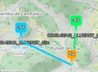
The network function is a legacy function which tests links to pre-calculated sites to reveal the strongest server(s) at the tested receiver site (eg. a customer’s house).
Request
The below example is a HTTP GET request for testing a location with receiver gain 2dBi and receiver height 2m to the BLUENET network. You must send your API key in the request header as normal.
https://api.cloudrf.com/network?lat=38.938322&lon=1.398755&net=BLUENET&rxg=2&rxh=2
Response
The response is a verbose JSON object containing metadata about each link tested. This can be parsed to reveal the required information eg. RSSI so you can plot coloured links for example:
[
    {
        "Engine": "Sleipnir 1.7.8",
        "Frequency MHz": 868,
        "Propagation model": "Egli VHF/UHF",
        "Model subtype": "Suburban",
        "Receiver": [
            {
                "Latitude": 38.93832,
                "Longitude": 1.398755,
                "Ground elevation m": 91,
                "Antenna height m": 2,
                "Receiver gain dBd": -0.15,
                "Receiver gain dBi": 2
            }
        ],
        "Transmitters": [
            {
                "Latitude": 38.94411,
                "Longitude": 1.399756,
                "Ground elevation m": 92,
                "Antenna height m": 2,
                "Distance to receiver km": 0.651,
                "Azimuth to receiver deg": 187.65,
                "Downtilt angle deg": 0.1,
                "Antenna gain dBd": 0,
                "Antenna gain dBi": 2.15,
                "Polarisation": "Vertical",
                "Power W": 1,
                "Power dBm": 32.15,
                "ERP W": 1,
                "EIRP W": 1.641,
                "ERP dBm": 30,
                "EIRP dBm": 32.15,
                "Free space path loss dB": 83.3,
                "Bandwidth MHz": 0.1,
                "Johnson Nyquist noise dB": 0.2,
                "Noise floor dBm": -115,
                "Channel noise dBm": -114.8,
                "Signal power at receiver dBm": -87.2,
                "Signal to Noise Ratio dB": 27.6,
                "Computed path loss dB": 117.2,
                "Model attenuation dB": 33.9,
                "Field strength at receiver dBuV/m": 50.9,
                "RX voltage 50 ohm dipole uV": 16,
                "RX voltage 50 ohm dipole dBuV": 24,
                "RX voltage 75 ohm dipole uV": 20,
                "RX voltage 75 ohm dipole dBuV": 26,
                "Raise RX antenna for LOS": 102,
                "Raise RX antenna for fresnel 60%": 313,
                "Raise RX antenna for full fresnel": 344,
                "Obstructions": [
                    [
                        38.93995,
                        1.399037
                    ],
                    [
                        38.94017,
                        1.399075
                    ],
                    [
                        38.94039,
                        1.399113
                    ],
                    ... snipped for brevity ...
                ],
                "Distance": [
                    0.012,
                    0.025,
                    0.037,
                    0.049,
                    0.062,
                    ... snipped for brevity ...
                ],
                "Terrain": [
                    102,
                    103,
                    108,
                    109,
                    112,
                    ... snipped for brevity ...
                ],
                "Terrain_AMSL": [
                    101,
                    102,
                    104,
                    108,
                    109,
                    ... snipped for brevity ...
                ],
                "Fresnel": [
                    0,
                    -2.04,
                    -2.86,
                    -3.47,
                    -3.96,
                    ... snipped for brevity ...
                ],
                "dBm": [
                    -21,
                    -31,
                    -38,
                    -42,
                    -46,
                    ... snipped for brevity ...
                ],
                "dB": [
                    51,
                    61,
                    68,
                    72,
                    76,
                    ... snipped for brevity ...
                ]
            }
        ],
        "Chart image": "https://api.cloudrf.com/API/archive/data?ppa=5d0ffce3&uid=1",
        "Network KML": "https://api.cloudrf.com/users/1/b7ce7077.kml",
        "Server ID": 8201612,
        "Server name": "0816143545_BLUENET_Site"
    },
    {
        "Engine": "Sleipnir 1.7.8",
        "Frequency MHz": 868,
        "Propagation model": "Egli VHF/UHF",
        "Model subtype": "Suburban",
        "Receiver": [
            {
                "Latitude": 38.93832,
                "Longitude": 1.398755,
                "Ground elevation m": 91,
                "Antenna height m": 2,
                "Receiver gain dBd": -0.15,
                "Receiver gain dBi": 2
            }
        ],
        "Transmitters": [
            {
                "Latitude": 38.94279,
                "Longitude": 1.386807,
                "Ground elevation m": 117,
                "Antenna height m": 2,
                "Distance to receiver km": 1.148,
                "Azimuth to receiver deg": 115.66,
                "Downtilt angle deg": 1.3,
                "Antenna gain dBd": 0,
                "Antenna gain dBi": 2.15,
                "Polarisation": "Vertical",
                "Power W": 1,
                "Power dBm": 32.15,
                "ERP W": 1,
                "EIRP W": 1.641,
                "ERP dBm": 30,
                "EIRP dBm": 32.15,
                "Free space path loss dB": 88.3,
                "Bandwidth MHz": 0.1,
                "Johnson Nyquist noise dB": 0.2,
                "Noise floor dBm": -115,
                "Channel noise dBm": -114.8,
                "Signal power at receiver dBm": -96.9,
                "Signal to Noise Ratio dB": 17.9,
                "Computed path loss dB": 126.9,
                "Model attenuation dB": 38.6,
                "Field strength at receiver dBuV/m": 41.3,
                "RX voltage 50 ohm dipole uV": 5,
                "RX voltage 50 ohm dipole dBuV": 14,
                "RX voltage 75 ohm dipole uV": 6,
                "RX voltage 75 ohm dipole dBuV": 16,
                "Raise RX antenna for LOS": 80,
                "Raise RX antenna for fresnel 60%": 92,
                "Raise RX antenna for full fresnel": 100,
                "Obstructions": [
                    [
                        38.93835,
                        1.398676
                    ],
                    [
                        38.93843,
                        1.398467
                    ],
                    [
                        38.93847,
                        1.398363
                    ]
                    ... snipped for brevity ...
                ],
                "Distance": [
                    0.01,
                    0.02,
                    0.03,
                    0.04,
                    0.05,
                    ... snipped for brevity ...
                ],
                "Terrain": [
                    111,
                    111,
                    110,
                    110,
                    110,
                    ... snipped for brevity ...
                ],
                "Terrain_AMSL": [
                    114,
                    112,
                    112,
                    111,
                    111,
                    ... snipped for brevity ...
                ],
                "Fresnel": [
                    0,
                    -1.85,
                    -2.61,
                    -3.18,
                    -3.65,
                    ... snipped for brevity ...
                ],
                "dBm": [
                    -16,
                    -27,
                    -34,
                    -39,
                    -43,
                    ... snipped for brevity ...
                ],
                "dB": [
                    46,
                    57,
                    64,
                    69,
                    73,
                    ... snipped for brevity ...
                ]
            }
        ],
        "Chart image": "https://api.cloudrf.com/API/archive/data?ppa=3a949f40&uid=1",
        "Network KML": "https://api.cloudrf.com/users/1/b7ce7077.kml",
        "Server ID": 8201611,
        "Server name": "0816143541_BLUENET_Site"
    }
]
HF Area
The /hf/area endpoint accepts a JSON object in the request body describing your network and will run a point-to-multipoint “heatmap” calculation using VOACAP.
Request
The below example is for a 4MHz signal at 00:00 UTC in July. The request is sent as a POST request to https://api.cloudrf.com/hf/area and it will return a JSON response containing metadata and URLs to image layers for your map.
{
    "site": "Test",
    "network": "HFTest",
    "transmitter": {
        "lat": 51.833992,
        "lon": -2.231319,
        "frq": 4.0
    },
    "antenna": {
        "txg": 2.0,
        "txl": 0.0,
        "ant": 1,
        "pol": "h",
        "azi": 90
    },
    "model": {
        "month": 7,
        "hour": 0,
        "rel": 50
    },
    "output": {
        "col": "SNR1.dB",
        "bounds": {
            "north": "72.499717",
            "east": "40.944650",
            "south": "6.353099",
            "west": "-60.400436"
        },
        "nf": -140,
        "out": 4
    }
}
Response
The PNG_Mercator image is warped for slippy maps like Mapbox, Leaflet and Google Maps. The PNG_WGS84 is for globes like Google Earth, Cesium and WinTAK.
{
    "kmz": "https://api.cloudrf.com/archive/M2JUbU5yOU5XNFFWZ29JZjNmaFFUdz09/kmz",
    "PNG_Mercator": "https://api.cloudrf.com/output/projection/3857/1/1017080906_HFTest_Test_HF",
    "PNG_WGS84": "https://api.cloudrf.com/users/1/1017080906_HFTest_Test_HF.4326.png",
    "bounds": [
        72.499717,
        40.94465,
        6.353099,
        -60.400436
    ],
    "id": 2025,
    "sid": "M2JUbU5yOU5XNFFWZ29JZjNmaFFUdz09",
    "key": [
        {
            "l": "40dB",
            "r": 37,
            "g": 131,
            "b": 255
        },
        {
            "l": "30dB",
            "r": 49,
            "g": 254,
            "b": 127
        },
        {
            "l": "20dB",
            "r": 218,
            "g": 254,
            "b": 60
        },
        {
            "l": "10dB",
            "r": 254,
            "g": 72,
            "b": 72
        }
    ],
    "elapsed": 2364.0,
    "balance": 10000000000
}
PNG image with colours which map to the signal levels in the JSON output:

HF Prediction
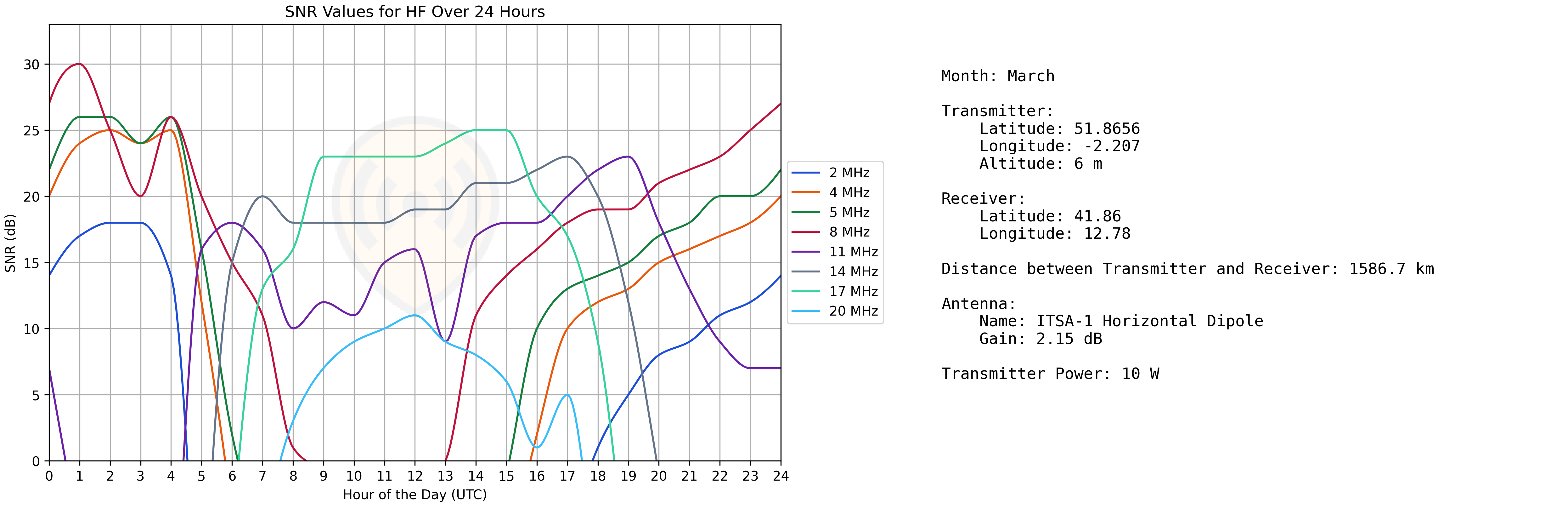
The /hf/prediction endpoint accepts a JSON object in the request body describing your network and will run a point-to-point calculation using VOACAP.
It produces an output for multiple frequencies, and so can be used for frequency selection.
Request
The below example is for a 4MHz signal in March. The request is sent as a POST request to https://api.cloudrf.com/hf/prediction and it will return a JSON response containing a link to a chart png.
{
    "site": "Test",
    "network": "HFTest",
    "transmitter": {
        "lat": "51.8656",
        "lon": "-2.207",
        "frq": 4.0,
        "txw": 10,
        "alt": 6.0
    },
    "receiver": {
        "lat": "41.86",
        "lon": "12.78",
        "rxg": "2.15"
    },
    "antenna": {
        "txg": 2.15,
        "ant": 2
    },
    "model": {
        "month": 3,
        "sunspots_r12": 50
    },
    "output": {
        "nf": -140
    }
}
Response
{
    "Transmitters": [
        {
            "Latitude": 51.8656,
            "Longitude": -2.207
        }
    ],
    "Receiver": [
        {
            "Latitude": 41.86,
            "Longitude": 12.78
        }
    ],
    "Chart image": "https://api.cloudrf.com/users/1/1029125124_HFTest_Test_HF_PPA.png",
    "elapsed": 1295.0,
    "balance": 10000000000,
    "metadata": {
        "locations": {
            "transmitter": {
                "latitude": 51.8656,
                "longitude": -2.207,
                "altitude_m": 6.0
            },
            "receiver": {
                "latitude": 41.86,
                "longitude": 12.78
            },
            "distance_km": 1586.7
        },
        "antenna": {
            "name": "ITSA-1 Horizontal Dipole",
            "gain": 2.15
        },
        "month": "March",
        "power_w": 10.0
    },
    "hours": {
        "hour0": [
            {
                "frequency": 2.0,
                "snr": 14.0
            },
            {
                "frequency": 5.0,
                "snr": 22.0
            },
            {
                "frequency": 8.0,
                "snr": 27.0
            },
            {
                "frequency": 11.0,
                "snr": 7.0
            },
            {
                "frequency": 14.0,
                "snr": -32.0
            },
            {
                "frequency": 17.0,
                "snr": -77.0
            },
            {
                "frequency": 20.0,
                "snr": -76.0
            },
            {
                "frequency": 4.0,
                "snr": 20.0
            }
        ],
        "hour1": [
            {
                "frequency": 2.0,
                "snr": 17.0
            },
            {
                "frequency": 5.0,
                "snr": 26.0
            },
            {
                "frequency": 8.0,
                "snr": 30.0
            },
            {
                "frequency": 11.0,
                "snr": -6.0
            },
            {
                "frequency": 14.0,
                "snr": -74.0
            },
            {
                "frequency": 17.0,
                "snr": -74.0
            },
            {
                "frequency": 20.0,
                "snr": -73.0
            },
            {
                "frequency": 4.0,
                "snr": 24.0
            }
        ],
        ...snipped for brevity...
    }
}
Chart image showing which frequencies are stronger at different times of day:
Area API with Bounded Output
Often the study area is far away from the transmitter, for example a suburb which is served by a mountain repeater. By bounding the output area in the request, only this focus area is computed and returned.
Aside from being very fast and efficient, it allows for higher resolution calculations than would be possible by testing the entire town / valley in all directions.
For example, to test an airfield with LiDAR accuracy that is 42km away from the transmitter you would populate the “bounds” array within the “output” section of an area request.
{
  ... snipped for brevity ...
    "output": {
        "units": "m",
        "col": "3",
        "out": "2",
        "nf": "-120",
        "res": "2",
        "rad": "42",
        "bounds": {
            "north": 51.677,
            "south": 51.655,
            "east": -2.039,
            "west": -2.076
        }
    }
}
More Information
For a complete OpenAPI 3 schema of the CloudRF API please consult the OpenAPI documentation.
Compression
CloudRF uses gzip compression for output files. The official client handles this but if you are writing your own you should use the MIME type rather than writing raw data as a .tiff may actually be .tiff.gz.
Below shows an example of this in Python 3:
# WARNING: Will write a gzipped file
shutil.copyfileobj(response.raw, outputFile)

# Will handle gzip decompression
outputFile.write(response.content)
Verbose Environment Variables
Since v3.8, the environment block has been redesigned to replace the cryptic cll and clm values with simpler boolean layers describing elevation, landcover, buildings and obstacles. This enables easier layering of custom clutter upon DTM for example (elevation = 2, obstacles = 1).
Both methods are supported in 3.8 but the long form is now the standard, as used in the web interface, and the old trigraph method is deprecated. It still features in places such as templates.
The following table translates old to new values:
Legacy Value |
New Value (3.8) |
|---|---|
cll = 0 |
landcover = 0 |
cll = 1 |
landcover = 1 |
cll = 2 |
landcover = 1, buildings = 1 |
clm = 0 |
obstacles = 0 |
clm = 1 |
obstacles = 1 |
clm = 2 |
elevation = 2, obstacles = 1 |
API Scripts
A list of ready-to-use scripts are available on the CloudRF public GitHub repository.
Some radio templates are here to help you pick good settings for hardware:
Demo gallery
There are interactive API demos on CloudRF’s public Github site hosted at https://cloud-rf.github.io/CloudRF-API-clients/gallery/
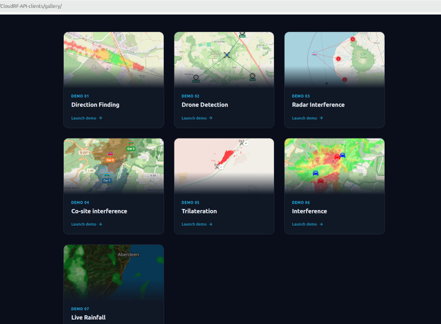
Unlike blog posts, these are live, browser-based tools, not articles. Each one lets a visitor interact with a map, change settings, and see a live request and response from CloudRF’s API. Visitors are welcome to reuse the example code from these demos in their own projects.
1. Direction Finding Demo
What it does: Shows how the API can enhance a single DF sensor to estimate where a signal may be located along a line-of-bearing (LoB).
How to use it: Drag a sensor icon to reposition it on the map, then click anywhere on the map to draw a Line of Bearing (LoB) — a direction pointing towards a possible transmitter. A “Recalculate” button reruns the analysis.
Default settings shown: 450 MHz frequency, a sensor 10 metres above ground, a transmitter power of 4 watts, and a 10-degree bearing arc (the margin of directional error).
What it demonstrates: This is a browser version of the direction-finding (DF) work covered in CloudRF’s “Enhancing Radio Direction Finding with RF Simulation” blog post — using simulation to narrow down a search area from a single bearing, rather than needing multiple sensors.
2. Drone Detection Demo
What it does: Simulates detecting a moving drone using multiple ground sensors. This is useful for effective siting of a system in a location without operator training.
How to use it: Drag the drone icon or the sensor icons to set their positions, adjust the drone’s altitude, and press “Calculate” to see which sensors would detect the drone and at what signal strength (RSSI). There’s also an “Autopilot” mode that flies the drone in a figure-eight pattern automatically, with an adjustable altitude range and number of loops. Results can be recorded and exported as a KMZ file (a format used by mapping tools like Google Earth).
Default settings shown: A drone altitude of 50 metres and a detection threshold of -95 dBm (a typical weak signal).
What it demonstrates: This is a hands-on version of the sensor-placement planning described in CloudRF’s “Optimising Drone Detection with RF Simulation” blog post — showing how multiple sensors combine to track a moving target.
3. Radar Interference Demo
What it does: Shows how a ship’s radar can interfere with nearby wireless internet networks in the RF Spectrum — and how safety systems respond.
How to use it: Drag a ship icon or click the map to position a radar source, then press “Show Radar Coverage” to see how far its signal reaches. A “Load WISP Coverage” button adds a wireless internet network to the map so the two can be compared. An animated track option (at 1, 3, or 5 seconds per step) moves the ship along a route automatically, similar to a real voyage.
Default settings shown: A coverage mode based on a -64 dBm Dynamic Frequency Selection (DFS) threshold — the point at which nearby wireless equipment is required to switch channels or shut down to protect the radar.
What it demonstrates: This is the interactive version of the case study in CloudRF’s “How a Passing Warship Took Out a Town’s Internet” blog post, referenced directly in that article as a tool built with the help of Claude.
4. Co-site Interference Demo
What it does: Simulates several radios operating near each other on neighbouring UHF channels.
How to use it: Drag car icons to set their real-world positions (the default map area is Eifel, Germany), choose from three close frequencies (462, 464, and 466 MHz), and press “Calculate.” A results table shows, for each radio, what percentage of its coverage area suffers interference on each frequency. Clicking a table cell reassigns that radio to a different frequency, so users can test different combinations.
Default settings shown: PMR (Private Mobile Radio) equipment transmitting at 2 watts.
What it demonstrates: How to plan frequency assignments for a group of radios working in the same area (known as “co-site” operation) so they don’t interfere with each other. This is a common real-world problem for event organisers, security teams, and emergency services sharing a small patch of spectrum and proves that more than a guard channel is needed.
5. Trilateration Demo
What it does: Shows how three radio sensors can narrow down the likely location of a signal source, using a method called trilateration aka multilateration.
How to use it: Adjust the received signal strength (RSSI) sliders for three towers (Rx A, Rx B, and Rx C) to see the search area shrink as more information is added. Three ready-made example scenarios are included: a signal near Tower A (a small ~0.1 km² search area), a signal on a road midway between towers (~4.7 km²), and a signal near Tower B (~1.9 km²).
Default settings shown: All three receivers start at -90 dBm, modelled at 800 MHz.
What it demonstrates: Unlike the single-sensor Direction Finding demo, this shows how combining readings from three fixed towers can pinpoint a location much more precisely than one bearing alone.
One of the demos has a false positive with multiple results. This is normal when working with simulation error as several locations will meet the criteria. If the error is too low, it may miss the real location. Too high and it won’t be helpful.
6. Interference Demo
What it does: Models how radios can interfere when several are operating close together. In this demo, they are on the same channel which is obviously not ideal but channels are reused when they are in different areas. The separation is where planning comes in.
How to use it: Drag car icons to reposition “signal” radios (shown in blue) and “noise” radios (shown in red), then press “Calculate Interference.” Dragging a car can also trigger an automatic recalculation.
Default settings shown: PMR446 radios (a licence-free walkie-talkie band) at 446 MHz and 2 watts, using CloudRF’s combined Multisite and Interference API.
What it demonstrates: A general-purpose view of how unwanted radios (noise sources) reduce the usable coverage of wanted radios (signal sources) — useful for understanding interference in crowded radio environments like events, warehouses, or shared frequencies.
7. Live Weather API Demo
What it does: Shows how rainfall affects radio coverage, using live weather data from XWeather’s API.
How to use it: Drag the transmitter to a location, choose a rainfall model, set a frequency and attenuation factor, and press “Calculate.” A “Refresh Rain” button pulls in current live rainfall data to recompute coverage under real, up-to-date weather conditions.
Default settings shown: 30 dBi antenna gain, 4 GHz frequency, an attenuation factor of 0.50, and a choice between a custom rainfall model or the ITU-R P.838-3 standard (an international model for predicting how rain weakens radio signals).
What it demonstrates: How higher frequencies (like 4 GHz) can be significantly affected by rain, and how CloudRF can combine live weather data with radio simulation for more realistic, real-time coverage predictions.
Summary table
# |
Demo |
Core method |
Related blog post |
|---|---|---|---|
1 |
Direction Finding |
Single-sensor bearing + simulation |
Enhancing Radio Direction Finding with RF Simulation |
2 |
Drone Detection |
Multilink detection across several sensors |
Optimising Drone Detection with RF Simulation |
3 |
Radar Interference |
Radar coverage vs. wireless network, DFS threshold |
How a Passing Warship Took Out a Town’s Internet |
4 |
Co-site Interference |
Frequency clash checking for co-located radios |
— |
5 |
Trilateration |
Three-tower signal narrowing |
— |
6 |
Interference |
Signal vs. noise radio modelling |
— |
7 |
Live Weather |
Rain-fade modelling with live weather data |
— |
Troubleshooting
The most common reasons for API support tickets are below.
Commas instead of decimals in floating point numbers eg. 446,000
Missing columns or rows in CSV data
Rate limiting errors triggered by a small radius and large resolution. Eg. 1km at 90m
Bad antenna name eg. dypole vs DIPOLE.ADF
For automatic processing in the UI, the CSV field must match a form input in the interface. Eg.
dbmshould beReceived Power (dBm)