Common Tasks

The following are instructions for completing several common tasks in radio engineering. They are intended as a guide only. For detailed instructions on each component see the relevant documentation section.

Measure the Coverage of a WISP Tower

A WISP tower is going to be built and evidence is needed to justify the cost/benefit.

1. Create the Tower Coverage

Create the tower coverage as a layer using the interface. If the antenna pattern is known then use that for the most accurate model, otherwise you can use custom beamwidth values from the datasheet.

2. Upload Zip Code Data for Properties

Prepare a CSV spreadsheet for the area containing zip codes. These can be grouped by streets or neighbourhoods and the zip or address is the unique value in the id column.

Example Property Data

latitude	longitude	id	group
51.8668	-2.2066	GL43HX	Barnwood
51.8641	-2.2129	GL43HY	Barnwood

3. Download the Results

You can download results as CSV by clicking the download button in the bottom left analysis window. This download will show you if a property is covered or not with a YES or NO. If your input data can be sorted and contains the same number of rows as the output, you can paste the YES/NO column into your input CSV for a very granular report into neighbourhood coverage.

Model Multiple Sites for Multiple Frequencies

The problem is how to efficiently model multiple locations but with different frequencies. The locations do not change.

1. Prepare a CSV Spreadsheet

Instead of entering locations manually into the user interface, enter them into a CSV spreadsheet to eliminate error with (repeat) siting. The format should as a minimum contain the fields latitude and longitude:

latitude	longitude
51.8668	-2.2066
51.8641	-2.2129

2. Save Radio Settings as Templates

Create your radio settings in the interface form and save them as a template. You will need a template for each frequency you need to test.

3. Import Data

Select a template for the first frequency eg. Frequency1, then using the data import “MANET tool” option, load in the CSV. Each site will be modelled with the chosen frequency and associated settings. Repeat by loading the next template, and loading in the same CSV.

Design a Network That Meets a Coverage Requirement

The requirement is for 95% coverage of a city with a LPWAN smart meter network. The network must be economical yet provide good coverage. The consultant must be able to demonstrate planned coverage meets the requirement.

1. Prepare Your Data

The most important aspect of this task is to prepare your data. You need CSV spreadsheets for the properties or locations you would like covered (maximum 60,000 rows per spreadsheet in the interface) and another for the gateway locations (maximum 1000 rows in the interface).

Pay particular attention to the site name and network name fields as these will be needed later when finding, deleting or analysing the data.

Example Property Data

latitude	longitude	id	group
51.8668	-2.2066	CloudRF	Barnwood
51.8641	-2.2129	Roundabout	Barnwood

Example Gateway Data

This verbose format is for the user interface “site import” feature only. If you choose to use the API directly, you can use any format so long as it conforms to the API at the point of request. Examples are here: https://github.com/Cloud-RF/CloudRF-API-clients/tree/master/python

Site,Latitude (degrees),Longitude (degrees),Transmitter Height (m),Receiver Height (m),Receiver Gain (dBi),Receiver Sensitivity (dBm),Frequency (MHz),Bandwidth (MHz),RF Power (W),Antenna Pattern,Antenna Polarization,Antenna Loss (dB),Antenna Azimuth (degrees),Antenna Tilt (degrees),Antenna Gain (dBi),Noise floor (dBm),Model,Measured units,Context,Diffraction,Reliability,Profile,Colour schema,Antenna Horizontal Beamwidth (degrees),Antenna Vertical Beamwidth (degrees),Front to back
Site 1,38.9053686786203,1.42393869858255,10,10,8,-50,446,1.4,30,OEM Half-Wave Dipole,V,0,240,10,8,-120,Egli VHF/UHF (< 1.5GHz),Received Power (dBm),Average / Mixed,Knife edge,50% / -0dB (Optimistic),Minimal.clt,RAINBOW,1,1,8
Site 2,38.9071885546264,1.43414926725016,11,1,10,-60,800,10,10,OEM Half-Wave Dipole,V,10,240,10,8,-90,Egli VHF/UHF (< 1.5GHz),Received Power (dBm),Average / Mixed,Knife edge,50% / -0dB (Optimistic),Minimal.clt,RAINBOW,1,1,8
Site 3,38.9045598298649,1.43757317051595,20,5,5,-70,2400,20,1,OEM Half-Wave Dipole,H,11,240,10,8,-70,Egli VHF/UHF (< 1.5GHz),Received Power (dBm),Average / Mixed,Knife edge,50% / -0dB (Optimistic),Minimal.clt,RAINBOW,1,1,8

2. Process the Gateway Data

Using either an API client or the new “site import” functionality in the user interface, push the CSV data into the API with the “Area” API. This could be CPU or GPU powered and will create heatmaps in your account for analysis. If you have labelled the network properly it will be easy to find the data in your archive.

3. Load the Data in the User Interface

Load the layers on the map by either clicking their names from your archive or merging them into a super layer using the super layer utility. If you processed the data using the MANET API this is unnecessary as the data is already a single layer.

4. Perform Coverage Analysis Using the Property Data

Import the CSV data containing customer properties using the Coverage Analysis import option and expect to see coverage results displayed in the bottom left corner. Results will report coverage as a percentage so 90% would be covering 9/10 properties in an area.

5. Move or Remove a Gateway

If a gateway needs changing to meet the requirement (95%), remove it from the network by selecting and deleting it in the archive and then do it again at the new location.

6. Download Results

You can download results as CSV by clicking the download button in the bottom left analysis window. This download will show you if a property is covered or not with a YES or NO. If your input data can be sorted and contains the same number of rows as the output, you can paste the YES/NO column into your input CSV for a very granular report into neighbourhood coverage.

Model HF NVIS Coverage

Enter an appropriate frequency between 2 and 8MHz and a Tx power in watts.
Choose the HF NVIS model in the model menu. The antenna will be automatically set although you may choose the azimuth and gain. Use 0dBi if you are not sure of the gain or it is a whip. Set diffraction off to reveal any shadows although it will likely diffract into them given the frequency.
Choose the context/height to match the scenario. If it’s day time then the D layer will be present but will attenuate low frequencies so bear this in mind. If it’s night time, use the F layer. If there’s uncertainty then use the E layer for a compromise.
For the receiver use 0dBi for a whip antenna.
Use the CPU engine with 180m resolution for links out to 200km. Otherwise use the GPU engine.
Click the map or press play or change a value like azimuth to trigger a calculation.

Find the Best HF Frequency for a Month

Choose the HF Skywave model in the model menu
Choose the month and hour
Set the sunspot number to match latest data (100 if unsure)
Use the path tool to click on the distant station on the map. The link chart will display showing the best frequencies to use for the link and time. If the chart is blank, there is nothing to show above 0dB SNR so you should consider your antenna, antenna height and power.

Model HF Skywave Coverage

From the “Model” menu select “HF Skywave”. This uses the VOACAP engine.
At the “Site/Tx” menu set your antenna height above the ground, eg. 6m.
At the “Signal” menu set your frequency and RF power. Default values of 10MHz and 30W will be set.
At the “Antenna” menu, choose your pattern and appropriate gain, eg. Horizontal Dipole, 2dBi.
At the “Mobile/Rx” menu set the threshold to -121dBm which is an S1 signal.
In the “Output” menu choose the HF S1-S9 colour schema.
Set the radius to reach your distant station eg. 2000km.
Click the green play button to model the HF area coverage.

If coverage is not showing, check you are using the HF colour key and your receiver threshold is at least -120dBm.

We have a series on videos for HF modelling on our YouTube Channel.

Model a Flight Path

Prepare your flight path as a KML linestring. These files can be exported from ADSB exchange.
Open the import dialog and choose “route analysis”. Load in the KMZ/KMZ.
The points should display on the map if a valid linestring was found.
Place and configure your ground station and click calculate to observe coverage along the flight path. If different altitudes are detected, the option to model a ground overlay will be removed so you only get coloured balls floating above the ground.

Test a Route for Coverage Against a Network

Route coverage analysis

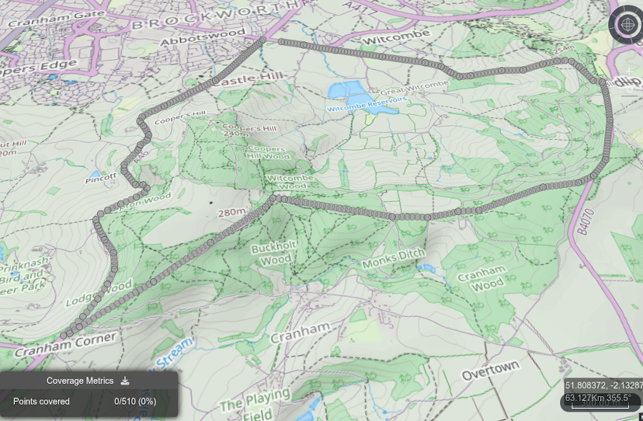
Create your route as a KML linestring in a suitable application, such as Google Earth or equivalent. Save it as KML or KMZ.
Import the KML/KMZ file using the file import dialog as “Coverage analysis”. Lots of grey points will be added to the map.
Create or reload a heatmap layer to test for coverage. The coverage will be reported in the coverage analysis dialog in the bottom left corner.
For a MANET network, enable the MANET tool and ensure heatmaps are enabled by clicking the donut icon in the MANET dialog. Links are ignored here. Place the MANET nodes by clicking upon the map.

Note that the settings for each node can be different but can only be defined prior to placing the node. Once placed, a node’s frequency and power cannot be changed but you can change global network values such as environmental settings.

See the Web Interface Import Data > Coverage Analysis section for more detail on this topic

Style Shapefile DN Values

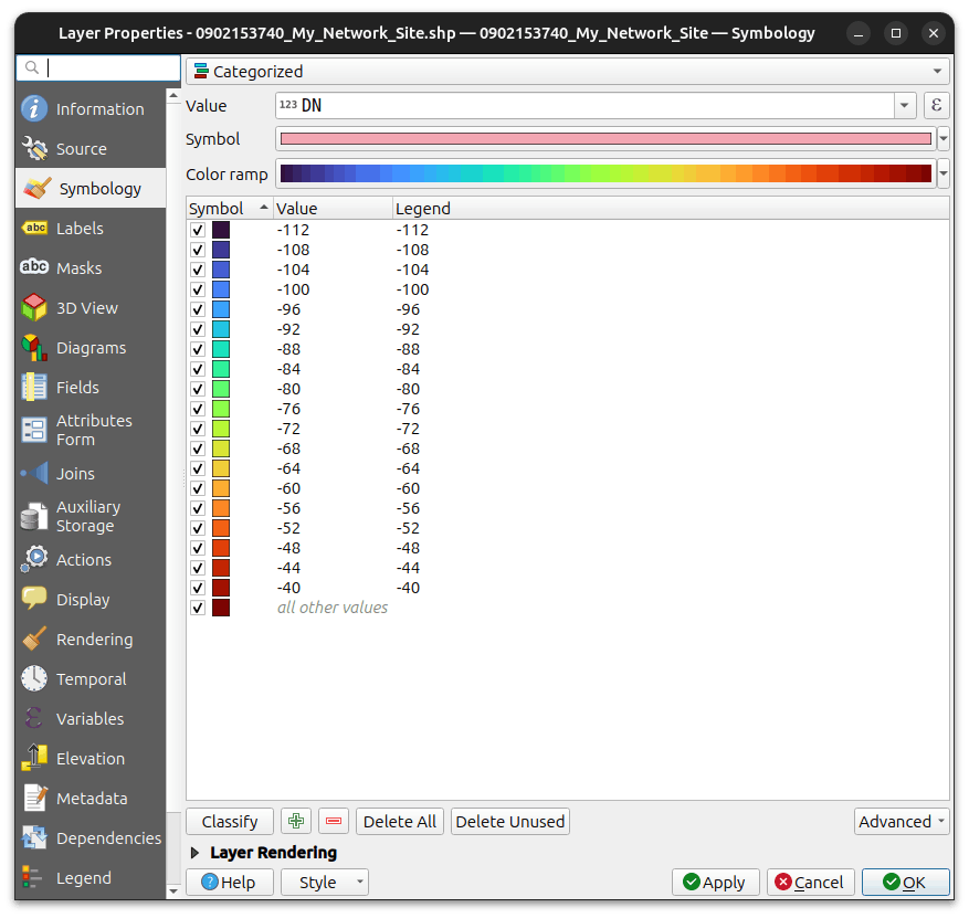
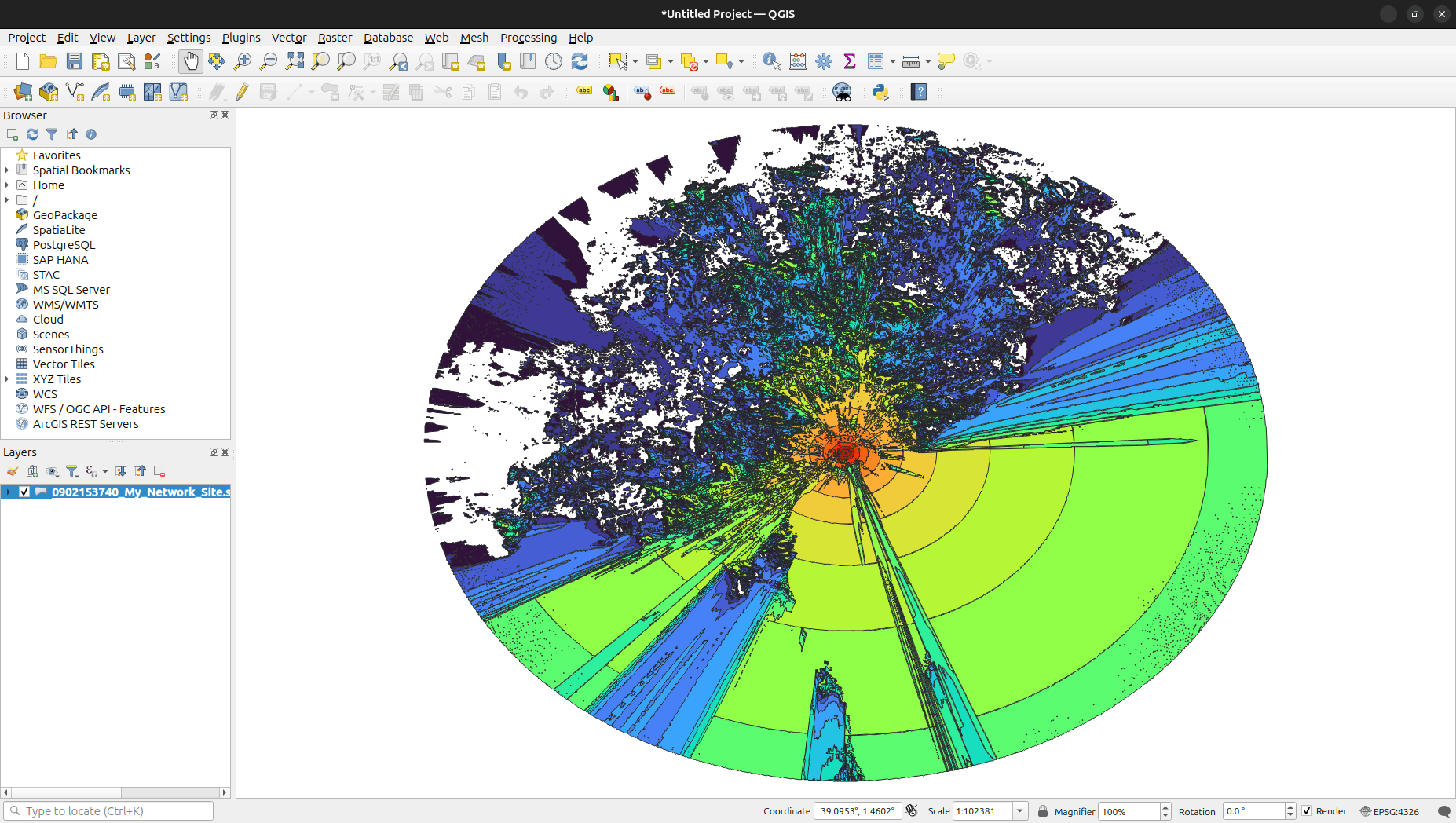
The ESRI Shapefile (SHP) contains embedded metadata to enable mapping of signal strength through to buckets within the calculated colour schema. These are represented as DN values within the Shapefile.

These can be loaded and referenced in other GIS software, such as QGIS, shown below to style to imported Shapefile in accordance with these DN values.

The API response contains RGB values for the requested colour key so buckets can be mapped directly to a signal level. Ensure your colour key has the range you need and if you want a 1dB granularity use the greyscale colour key.

QGIS Symbology

QGIS Styled SHP

A video tutorial for this is available on YouTube.

Build an RF tool with GenAI

The following suggested prompts will get you a mission-specific web-based tool using the correct API and enough information for an MVP. We recommend Claude which has proven to be good at digesting our Open API documentation.

Create a counter-drone planning tool which lets an operator place multiple sensors on a slippy map at configurable heights. 

Implement the CloudRF Multisite API to model the RF coverage of the sensors using a 2.4GHz frequency and provide a form to enter the API key.

To sharpen up the API settings:

For the Multisite call, use a green colour key, received power units with a -100dBm threshold and a receiver altitude of 50m above the ground

To add a Rural option with DTM:

Add a checkbox for rural mode which optimises Multisite API settings for the country. Output resolution should be 20m, Radius set to 10km, environment elevation to 2, buildings to 1, landcover to 1, Profile to "Temperate.clt".

To add a Urban option with LiDAR / DSM:

Add a checkbox for urban mode which optimises Multisite API settings for a City. Output resolution should be 2m, Radius set to 1km, environment elevation to 1, buildings to 0, landcover to 0.

Integration and testing

CloudRF’s API has been extensively field tested and integrated into different systems. This is a summary of our public blogs and their key findings.

1. Simulating Throughput

Posted: 28 August 2026

This post explains “throughput” — how much data a radio link can actually carry — and how CloudRF estimates it.

The basics:

Bandwidth — how much radio spectrum a channel uses. More bandwidth generally means more capacity, but it also lets in more background noise.
Signal-to-noise ratio (SNR) — how strong the signal is compared to the noise. A clean, strong signal supports “denser” data encoding and faster speeds; a weak or noisy signal forces the system back to slower, more robust methods. This is why a phone gets slower as you move away from a mast.

There’s a well-known formula (the Shannon-Hartley theorem) for the theoretical maximum speed of a link, but real systems never reach that maximum. CloudRF instead gives a deliberately cautious estimate, based on Wi-Fi-style standards, so that users are more likely to be pleasantly surprised than let down.

Case study — a large festival: The team modelled Wi-Fi coverage for a fictional set-up at Glastonbury Festival, which draws over 200,000 people:

Mapping basic coverage using terrain and building data.
Adding temporary structures (tents, stages) that aren’t in standard map data.
Testing throughput at two bandwidths (5 MHz and 20 MHz) — wider bandwidth gave faster speeds but slightly less coverage.
Re-testing with a much higher noise level, based on real readings from a previous year’s event, to see a “worst case” result.

Field test conclusions: This is a fictional planning case study, not a physical field test.

Technologies integrated: CloudRF’s throughput modelling feature, terrain and building data, custom/temporary structure modelling, real noise readings from previous events.

Bottom line: Throughput depends on both bandwidth and noise, doubling bandwidth doesn’t come free, and planning for realistic (even worst-case) noise conditions avoids nasty surprises on the day.

2. Autodesk Revit CloudRF Plugin

Posted: 6 August 2026

CloudRF built a plugin for Autodesk Revit, a building-design app. The plugin lets Revit users run radio signal simulations without leaving the app.

What it does:

Lets users place a transmitter and calculate radio coverage inside a 3D building model.
Supports configurable reflections and resolution down to 10 cm.
Models material properties like signal loss through walls and reflections.
Works with CloudRF’s cloud service or with SOOTHSAYER, a server you can run on your own premises.
Converts CAD (building design) files to glTF, a 3D file format, automatically in the background.
Can simulate multipath signals — where two versions of a signal arrive out of step and cancel each other out, causing “dead spots.”
Works with different wireless technologies, including private 5G, Wi-Fi, and COFDM (a type of digital radio signal).

Field test conclusions: None — this is a product/feature announcement, not a field test.

Technologies integrated: Autodesk Revit, SOOTHSAYER (on-premises server), glTF conversion.

Status: This plugin is still in early development (alpha stage). It is slower than CloudRF would like, mainly because of the file conversion step. CloudRF is inviting interested users to try it.

3. SignalHound Integration Field Test

Posted: 6 August 2026

CloudRF connected a SignalHound radio receiver to its system to try locating a hidden transmitter using drive-test data.

What they did: The team drove a short 1.5 km loop near some large buildings, collecting signal readings from a VHF radio tower about 2 km away. They then ran a “grid search” — testing thousands of possible locations to see which one best matched the readings.

Field test conclusions:

The tower’s likely location was correctly narrowed down, even though the drive route covered only a small range of angles.
The full search, covering many possible grid squares, took less than 5 seconds.

Technologies integrated: SignalHound radio receiver, CloudRF API (grid search using drive-test data).

Bottom line: This test showed that searching a grid of locations is a workable way to find a transmitter’s position, as long as the simulation is fast enough — and that publishing an open API makes it easy to add new hardware like this.

4. Tough Stump Rodeo 2026

Posted: 7 June 2026

CloudRF took part for the first time in the Tough Stump Rodeo, a field exercise in rural Montana. Teams had to set up communications from a headquarters (HQ) to an underground mine, 50 km away in mountainous terrain.

Preparation: The team gathered high-resolution terrain and tree-canopy data for the area weeks in advance and loaded it onto offline servers, since there would be no internet at the site.

Field test conclusions:

A site visit to the mine confirmed there was no background radio interference nearby, and identified a hill about 750 m away that offered a good relay point.
Simulation showed a relay could reach 35 km down the valley towards HQ, avoiding the need for extra equipment.
A tool called “bounds” let the team run detailed, focused simulations over long distances quickly, instead of slow, low-detail maps of the whole area.
Simulation matched what they found in the field: a weak first link improved once moved to higher ground, and a second relay position was fine-tuned using live software on-site.
A radio check from the mine was eventually heard clearly at HQ, 50 km away, over three relay hops.
On demo day, a live drone video feed from the mine worked well — until a crowded Wi-Fi signal inside the viewing tent caused it to briefly fail. It recovered automatically once the Wi-Fi switched to a clearer channel.

Technologies integrated: offline terrain and tree-canopy data servers, the “bounds” simulation tool, ATAK (including a live coverage map connected to a live radio network), on-site relay calibration software, live drone video feed integration.

Bottom line: Careful planning with simulation meant the team needed fewer relay stations and had no wasted trips to test bad locations — the field results matched the predictions closely.

5. How a Passing Warship Took Out a Town’s Internet

Posted: 30 April 2026

In July 2025, the Australian warship HMAS Canberra sailed past New Zealand’s coast with its navigation radar on. Nearby residents’ wireless internet stopped working, and the story went viral. CloudRF used its simulation tools to explain what actually happened.

The radar: The ship’s SAAB Sea Giraffe AMB radar operates in the C-band (around 5.5 GHz) — the same general range used by some 5G fixed wireless internet services. Full technical specifications aren’t public, so CloudRF estimated the missing details (power, height, bandwidth) from available photos and documents.

Key finding — Dynamic Frequency Selection (DFS): Wireless equipment in this frequency band is required, by international rules, to detect radar pulses and automatically switch channels or shut down to avoid interfering with the radar. CloudRF modelled the ship’s radar signal along its likely route and found the signal strength easily exceeded the DFS trigger threshold along much of the coastline — closely matching where outages were reported (and suggesting some unreported outages may also have occurred).

Conclusion: The internet outage was caused by wireless equipment automatically and correctly protecting the ship’s radar, not by physical jamming or damage. It worked as the safety system was designed to.

A deeper “what if” analysis: CloudRF also modelled what would happen without the DFS safety feature:

The radar signal would cause interference on nearby Wi-Fi-style channels beyond its own bandwidth — a wider effect than a simple frequency-range calculation would suggest.
In the other direction, modelling showed home wireless signals reaching the ship could raise the radar’s background noise significantly, which could reduce the radar’s detection range — a genuine safety risk, which explains why radar is prioritised.
CloudRF suggests visiting warships could avoid this by using radar frequencies away from civilian networks, or notifying local spectrum authorities in advance.

Field test conclusions: This is a desk-based simulation study reconstructing a real event, not a new physical field test. It draws on public reporting (RNZ, The Guardian) and a fictional but licence-realistic wireless tower model built by CloudRF.

Technologies integrated: CloudRF’s interference tool, Superlayer (a tool for combining multiple coverage results into one), and — noted directly in the post — Claude, used to help build a public interactive demo tool showing the radar/network interference.

6. Optimising Drone Detection with RF Simulation

Posted: 21 April 2026

This is a detailed guide on using CloudRF to plan where to place drone-detection and radar equipment.

The problem: Where you place a detection sensor matters a lot. In cities, tall buildings block signals. In open countryside, coverage is much better with the same equipment. Trees and forests cause similar problems. Background radio noise also changes with the time of day and nearby events.

The solution: CloudRF lets users build a “template” — a saved set of equipment settings — and test it against real terrain and building data. Key settings include height units (metres above ground for drones, feet above sea level for aircraft radar), model type (radar model for aircraft-style detection, standard model for drones), environment data (building maps, tree-height data, LiDAR), and noise (known level or live sensor readings).

Tools covered:

Best Site Analysis — automatically scores locations across an area to find the best spots for equipment.
Area Calculation — shows the coverage from a chosen site.
Best Server — checks which sensor in a network can “see” a target at a given position.

Case study conclusions:

A stadium in Texas: The team modelled where to place drone-detection sensors around a stadium. The stadium roof scored best, but blocked signal to the north. Adding a second sensor solved this.
Dartmoor, UK: Using one direction-finding sensor, the team narrowed down where a drone’s ground controller might be, even without multiple sensors to triangulate.

Technologies integrated: Best Site Analysis, Area Calculation, and Best Server tools; LiDAR terrain data; building maps; tree-height data; live and manual noise inputs.

Bottom line: Good sensor placement, checked with simulation before going into the field, saves time and improves detection coverage — especially in tricky environments like cities, forests, or hilly terrain.

7. Choosing an RF Propagation Model

Posted: 20 March 2026

This post explains how to pick the right radio propagation model — a formula that predicts how a radio signal weakens over distance. CloudRF tested several models against real-world measurements and gives a clear recommendation.

Headline conclusion: CloudRF now recommends ITU-R P.1812 as the default model for most users.

Background:

Propagation models fall into two types: deterministic models (formula-based, consistent results, e.g. ITM and P.1812) and empirical models (based on past survey data, e.g. Okumura-Hata, COST 231, Ericsson 9999).
Empirical models only work well if you correctly guess the environment type (urban, suburban, rural). Get that setting wrong, and the prediction can be badly off.
Terrain and clutter (buildings, trees, water) data quality has a big effect on accuracy, regardless of which model you choose.

Field test conclusions: CloudRF ran real-world comparisons across five frequency bands (41.5 MHz to 2.1 GHz) using data from broadcast towers, an LTE mast, and Arctic field tests in snow-covered terrain.

VHF broadcast (41.5–196 MHz): ITU-R P.1812 gave the most consistent, accurate results across three separate UK test sites. Free-space and older empirical models performed poorly or inconsistently.
UHF/LTE (800 MHz): Both the General Purpose model and ITU-R P.1812 gave good results (single-digit decibel error). Empirical models (Okumura-Hata, Ericsson 9999) only worked once the “environment context” setting was corrected to match the actual open, rural terrain.
LTE in snow (1820 & 2140 MHz): Tested near the Arctic Circle under snow-covered trees. ITU-R P.1812 and the older ITM model gave the closest match to real measurements at both frequencies. Newer high-frequency empirical models performed very poorly here.
Overall: ITU-R P.1812 was the most reliable model across every test, without needing manual tuning first. Older empirical models can still work well, but only with field data to calibrate them correctly.

Technologies/methods used: ITU dataset (Study Group 3), CloudRF’s calibration tool, machine-learning-assisted calibration (referenced for further reading).

8. Live Network Mapping Endurance Test

Posted: 11 February 2026

CloudRF tested its live network mapping system in the Scottish mountains. The goal was to see if the system could run all day, in the cold, on battery power.

What they did: The team walked a 16 km circular route at the Glenshee ski resort in temperatures of -10°C. They carried a small computer (an Nvidia Jetson) that ran radio coverage calculations and sent live updates to a phone running the ATAK mapping app. This setup lets a network map update itself automatically as people move, instead of someone building a map by hand.

Field test conclusions:

The system created 925 coverage maps and 4,625 signal-strength checks in one day.
Power use stayed low — around 7.5 watts, well within what a phone charger battery can supply.
A small 45-watt-hour battery lasted longer than a bigger 92-watt-hour one; the larger battery turned out to be faulty.
The test uncovered a bug: the app sometimes switched to the wrong height setting when GPS readings looked like the device was flying. This happened because GPS height readings can be off by more than 100 metres in hilly terrain. CloudRF turned this logic off and fixed the plugin.
They also found that ATAK’s own height data was inconsistent between different parts of the app.

Technologies integrated: Nvidia Jetson (edge computing), ATAK mapping app, GPS-based positioning.

Bottom line: The system proved it could run reliably all day on battery power in harsh conditions, and the team fixed a height-tracking bug that the test uncovered.

9. Enhancing Radio Direction Finding with RF Simulation

Posted: 25 November 2025

Radio Direction Finding (DF) locates a radio transmitter using a single sensor, which gives a “Line of Bearing” (LoB) — a direction, but not a distance. CloudRF tested whether adding RF simulation could narrow down the likely location along that line.

The problem: Without knowing a transmitter’s power, its possible distance can vary hugely — CloudRF’s example shows a signal could be 2.4 km or 15 km away, depending on assumed power. Simulation helps narrow this range by accounting for real terrain and clutter.

Field testing: CloudRF built and tested a portable DF rig combining a KrakenSDR direction-finding receiver (accurate to about 8 degrees), a Raspberry Pi 5 running CloudRF’s SOOTHSAYER software to generate simulation data at the edge (on-site, without internet), a CRFS RFEye receiver for accurate power measurements, Meshtastic LoRa GPS trackers to record the true test radio’s position, and ATAK (a tactical mapping app) for visualising results.

Field test conclusions:

Field tests in the rain were disrupted by local radio interference and limited battery life, so the team reused a richer existing dataset from a prior vehicle-based field test instead.
When the radio’s transmit power was known, simulation shrank the possible search area to an average of 7.93% of the original area.
Even when the power was unknown, simulation still reduced the search area to an average of 31.51% of the original — roughly a two-thirds reduction.
The benefit depended on terrain: a clear, uniform obstacle (like a single forest) gave a tight, accurate probability band. Areas with multiple obstacles (hills plus forest) produced some false positives a human analyst could still rule out.
Conclusion: Adding simulation meaningfully improves the usefulness of a single line of bearing — but only if the analysis is automated, since doing it manually would be slower than a traditional map study.

Technologies integrated: KrakenSDR, CRFS RFEye, Raspberry Pi 5, SOOTHSAYER, Meshtastic LoRa trackers, ATAK, CloudRF API.

10. Fast Simulation Calibration with Machine Learning

Posted: 24 September 2025

This post compares real-world radio surveys with computer simulation, and introduces a machine-learning tool that speeds up matching the two.

The core trade-off: Physical surveys (drones, drive-test vehicles, or someone walking around with phones) are more accurate than simulation, but far slower and more resource-intensive.

A basic empirical model like Hata gives about 8 dB of accuracy.
Calibrated survey equipment can reach about 2 dB.
A standard phone app can reach about 3 dB.

Manual calibration: CloudRF’s web interface already lets users manually adjust model and clutter settings until simulated results match survey measurements. A good result is under 8 dB of error. This works but takes engineer time and is repetitive.

The “pizza problem”: Often, a customer only has survey data for part of a site (a “slice”), not the whole area, due to lack of time, access, or resources. The limited data must then be used to estimate the rest.

New tool — a genetic algorithm: CloudRF built an automated machine-learning tool that:

Takes a slice of real survey data.
Repeatedly tests different combinations of settings (like building attenuation, tree height, and tree signal loss) against CloudRF’s Area API.
Scores each attempt using Root Mean Square Error (RMSE), a measure of how far off the prediction is.
Breeds the best-performing settings into the next round, repeating until it converges on the most accurate settings.

Field test conclusions: No independent field test is reported — the tool is validated conceptually using existing survey data (from partner Rantcell), not a new physical field test.

Technologies integrated: CloudRF Area API, rasterio (a geospatial imaging library), SOOTHSAYER (for edge/offline use), Rantcell survey app data.

Future integration ideas raised: live coverage maps paired with spectrum analysers, signal classifiers, real-time antenna adjustment feedback, and autonomous robots that update coverage maps as they move.

11. Improving Accuracy in the Trees

Posted: 3 July 2025

CloudRF improved how its simulation engines calculate signal loss through obstacles like trees and buildings, leading to better accuracy and faster performance.

Headline results:

20% accuracy improvement when clutter (trees, buildings) is included in a simulation.
6.8 dB average error for non-line-of-sight simulation, a 1.6 dB improvement.
78% faster GPU processing when clutter is enabled.
Better modelling for radios operating underneath tree cover.

What changed: Previously, the engine had to choose between two effects when a signal met an obstacle: attenuation (loss passing through it) or diffraction (bending over the top). The system used to apply different logic to different obstacle types — treating a forest as something the signal diffracts over, and a building as something it attenuates through. This caused visual glitches and meant users had to choose between seeing rooftop signal levels (using detailed LiDAR height data) or in-obstacle signal levels — not both together. The new version calculates both effects together, consistently.

How to calibrate vegetation loss (method shared in the post):

Find two similar radio paths — one going through a uniform patch of trees, one going beside it in the open.
Calibrate the model so the clear (open) path matches real measurements.
Measure the extra signal loss on the obstructed path.
Divide that loss by the depth of the trees to get a loss-per-metre figure for that vegetation type.

Typical vegetation loss ranges from 0.03 to 0.5 dB per metre, depending on vegetation type and density.

Field test conclusions: CloudRF validated the update using real OFCOM UHF 450 MHz spectrum data from a coastal city — over 10,000 vehicle-collected samples covering hills and forest.

Test	Old engine	New engine
GPU, with clutter	11.7s, 8.4 dB error	2.6s, 6.8 dB error
CPU, with clutter	24.1s, 9.2 dB error	33.7s, 7.4 dB error

The GPU version got both faster and more accurate. The CPU version got more accurate but slightly slower when clutter was enabled. Simulations without clutter, or using rooftop-only mode, are unaffected.

Planned next step: CloudRF said it would run a dedicated field test collecting VHF/UHF attenuation data from inside an actual forest, to further refine default vegetation settings.

Technologies/data integrated: ITU-R P.833 (international standard for vegetation/material attenuation values), ESA Worldcover (satellite land-cover data), OFCOM UHF spectrum survey data, GPU (RTX 3050) and CPU (Ryzen 9) benchmarking.

12. Mapping Noise

Posted: 23 May 2025

Radio “noise” is interference that makes it harder to receive a clear signal. This post explains how CloudRF’s approach to modelling noise has improved over time.

2022: Users entered one noise number to represent an entire area. This was a rough guess.
2023: CloudRF added a way to store real noise readings for each site, so different locations could have different noise levels.
2025: CloudRF built a full noise map — a detailed layer showing noise at thousands of points across an area, down to 12-metre detail. This can use live sensor data, so the map updates as real conditions change.

Field test conclusions: None reported directly — this post traces a three-year feature evolution rather than a single field test.

Technologies integrated: DORA, an open-source project using low-cost radio receivers (around £200 each) to collect real noise readings and feed them into CloudRF; per-site noise storage; live sensor data feeds.

Bottom line: Noise varies by location and changes over time. CloudRF’s tools have moved from a single guessed number to a detailed, and even live, map of real interference.

13. The Art of HF

Posted: 16 April 2025

This post introduces a 3-part video series on HF (high-frequency) radio, which can send signals over 1,000 km using very little power by bouncing them off the upper atmosphere.

Frequency selection: the best frequency to use changes throughout the day and night. CloudRF’s tools can show which frequency gives the best signal-to-noise ratio at any given hour.
Antenna basics: covers the half-wave dipole antenna, including how to calculate its length, how mounting height affects performance, why the antenna must be aimed correctly, and how cable choice affects signal loss.
Forecasting: solar activity (measured by the “sunspot number”) affects how well HF signals travel, and this can be predicted and planned for.

Field test conclusions: None — this is a video series introduction, not a field test report.

Technologies/tools referenced: CloudRF frequency-selection tools, dipole antenna calculator, solar activity (sunspot) forecasting.

Bottom line: With the right frequency, timing, and antenna setup, HF radio can achieve very long-range links on minimal power — and CloudRF’s tools help predict the best conditions.

Summary table

#	Post	Date	Field test?	Key technology/integration	Headline conclusion
1	Simulating Throughput	28 Aug 2026	No (case study)	Throughput modelling, festival case study	Bandwidth and noise both shape real-world speed
2	Revit Plugin	6 Aug 2026	No	Autodesk Revit, SOOTHSAYER, glTF	Alpha-stage plugin for in-app RF simulation
3	SignalHound Integration	6 Aug 2026	Yes	SignalHound receiver, grid search API	Transmitter location narrowed via grid search in <5s
4	Tough Stump Rodeo 2026	7 Jun 2026	Yes	Offline servers, “bounds” tool, ATAK	50km link achieved over 3 relay hops; fewer relays needed than planned
5	Warship Internet Outage	30 Apr 2026	No (event reconstruction)	Interference tool, Superlayer, Claude	Outage was DFS working correctly, not jamming
6	Optimising Drone Detection	21 Apr 2026	Case study	Best Site Analysis, LiDAR	Second sensor fixed stadium blind spot; DF narrowed search on Dartmoor
7	Choosing a Propagation Model	20 Mar 2026	Yes	ITU dataset, calibration tool	ITU-R P.1812 recommended as default model
8	Live Network Mapping Endurance Test	11 Feb 2026	Yes	Nvidia Jetson, ATAK	System ran all day in -10°C; height bug found & fixed
9	DF with RF Simulation	25 Nov 2025	Yes	KrakenSDR, RFEye, Pi 5, SOOTHSAYER, ATAK	Simulation cut DF search areas by up to ~92%
10	Fast ML Calibration	24 Sep 2025	No	CloudRF API, rasterio, Rantcell data	Genetic algorithm automates model calibration
11	Improving Accuracy in the Trees	3 Jul 2025	Yes	ITU-R P.833, ESA Worldcover, OFCOM data	20% accuracy gain, 78% faster GPU processing
12	Mapping Noise	23 May 2025	No	DORA low-cost sensors, live noise maps	Noise modelling evolved from a guess to a live map
13	The Art of HF	16 Apr 2025	No	Frequency/antenna/solar tools	HF video series on long-range, low-power links