The rapid growth of Counter Unmanned Aerial Systems (C-UAS) across government, public, and commercial sectors has increased the need for accurate modelling to improve sensor siting and effectiveness.
This blog explores how Counter- (C-UAS) and RADAR systems can be modelled efficiently within CloudRF to optimise siting and improve their effectiveness.
The challenge
The methodology for operating sensors varies depending on the environment in which they are operating:
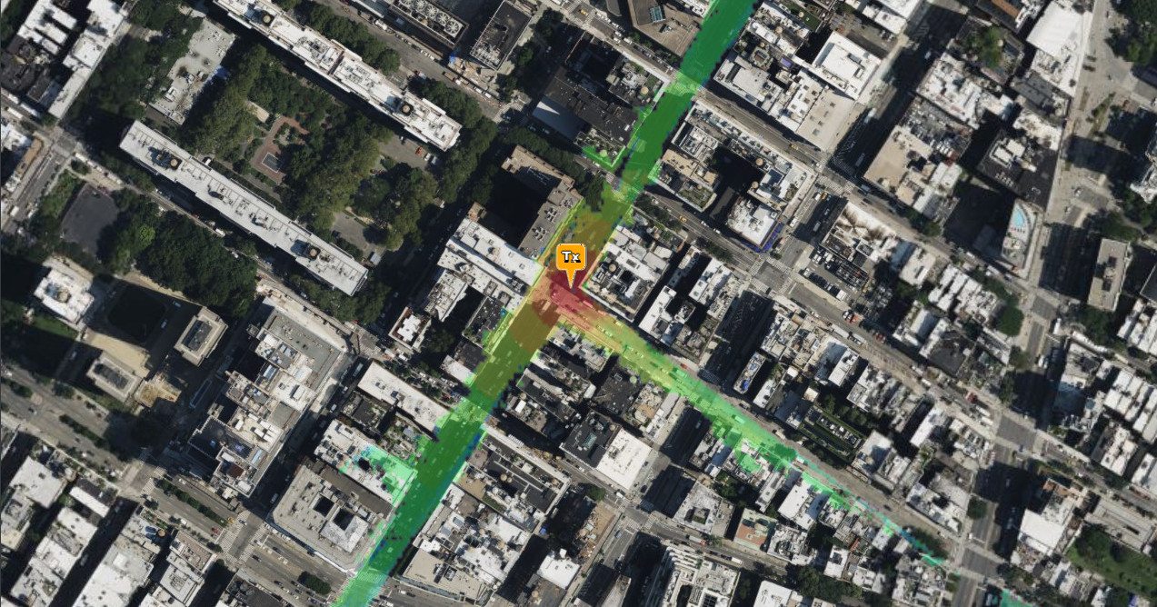
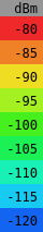
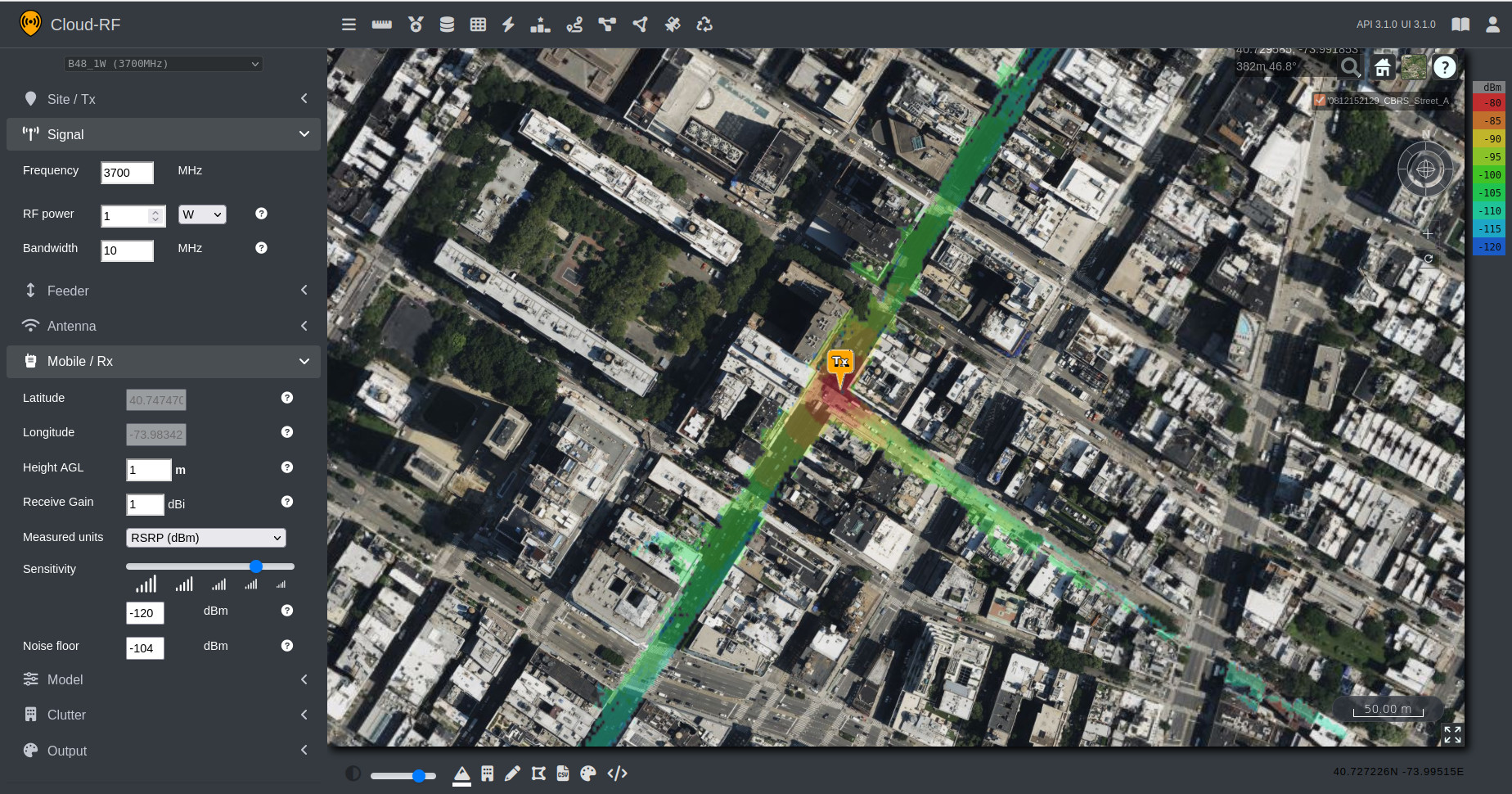
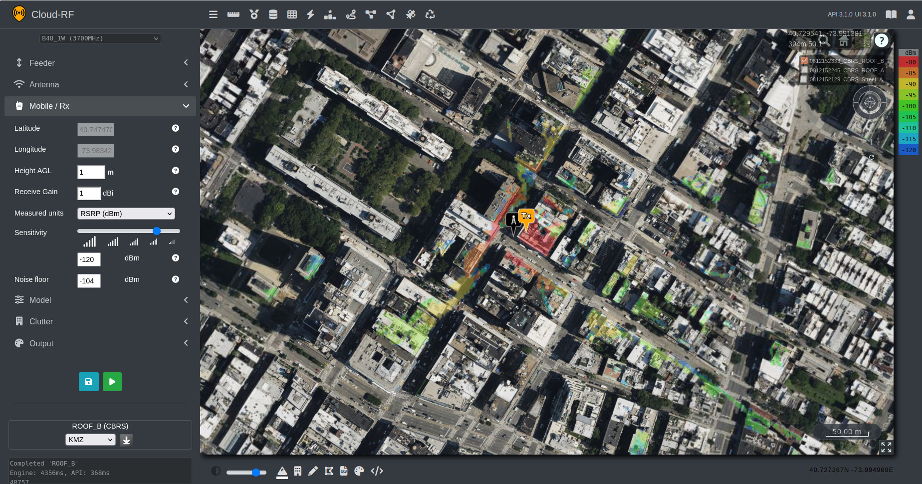
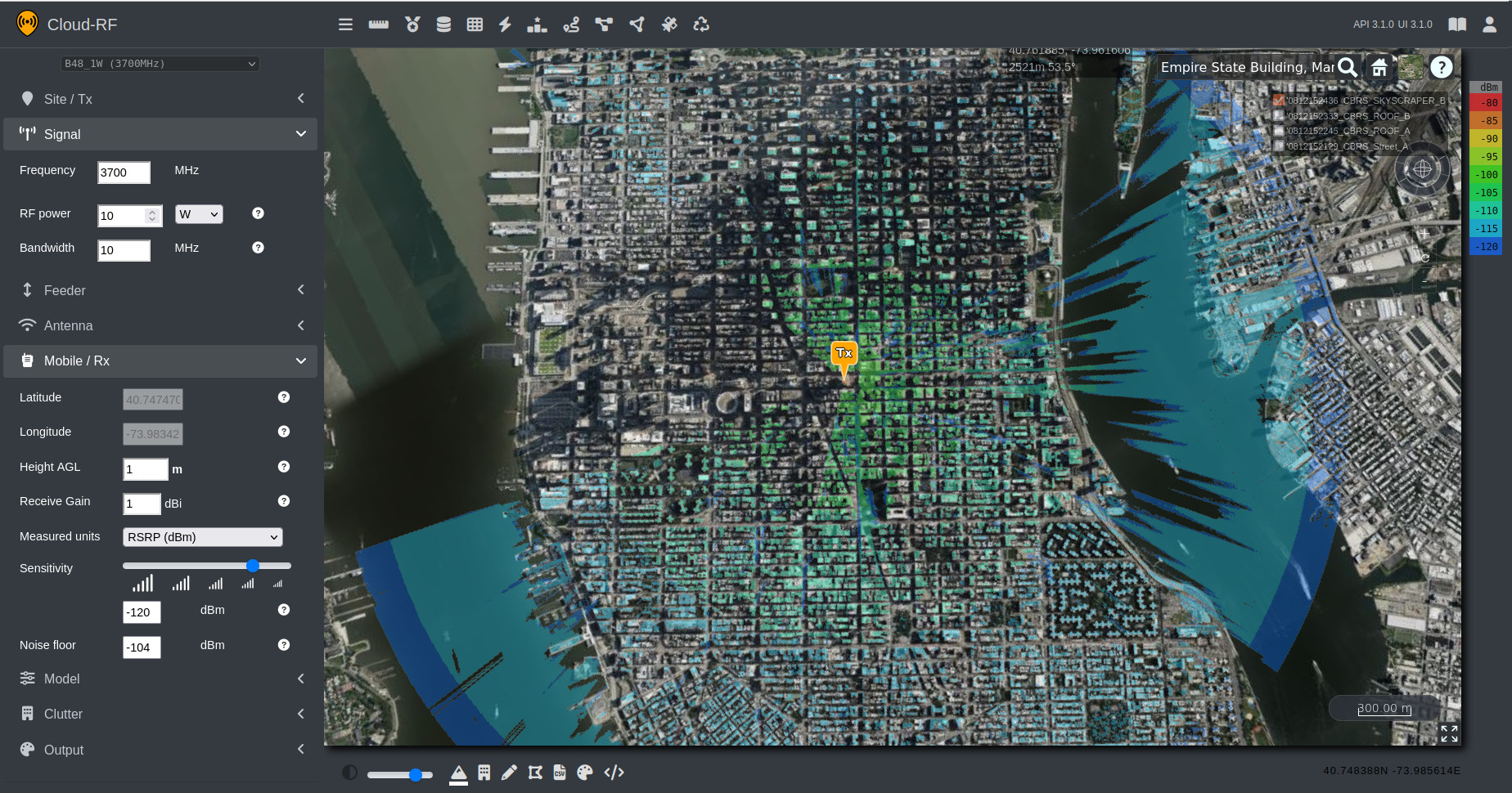
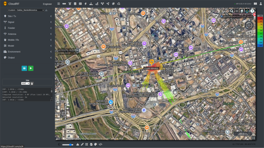
In dense urban environments, high-rise buildings reduce Line Of Sight (LOS) and block ultra high frequency signals, creating what are commonly referred to as urban canyons. An example of this effect for a poorly sited sensor at street level is shown in the screenshot below. In such environments, reliable coverage is limited to areas where a clear Line-Of-Sight (LOS) path exists.
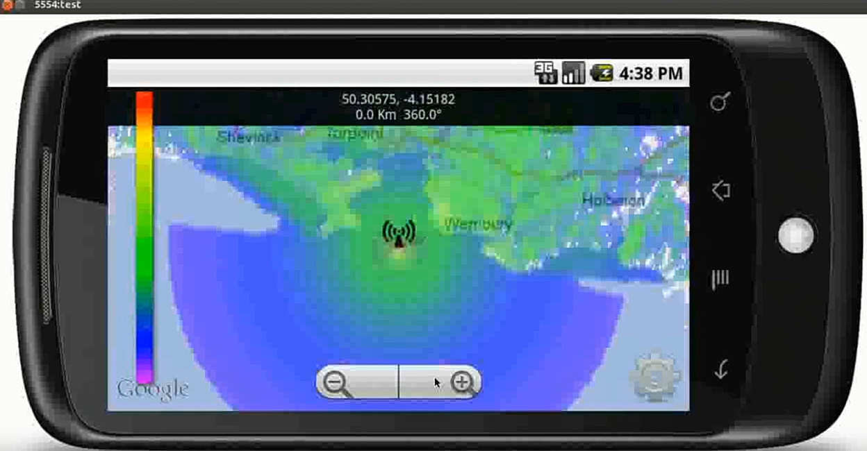
By contrast, in open rural environments, where terrain and structural obstructions are minimal, significantly greater and more consistent coverage is achieved using the same transmitter configuration. This comparison highlights the substantial impact that the environment has upon system performance.
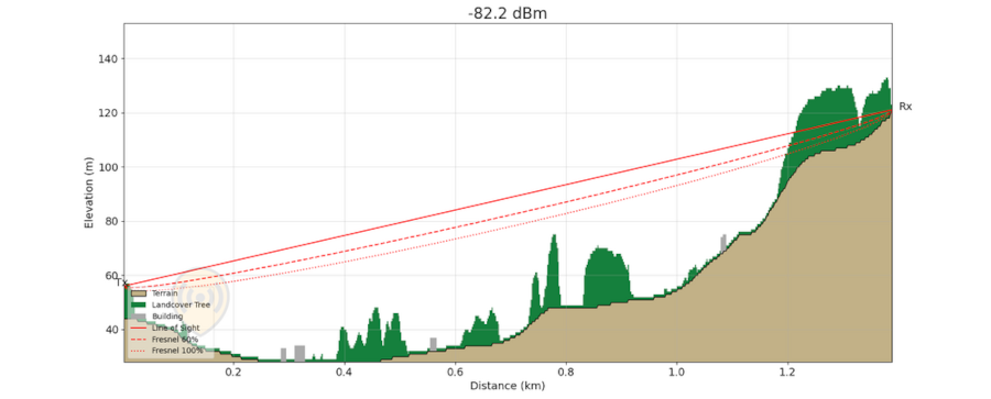
Similar challenges arise in environments where vegetation screening is present, particularly in forested and jungle regions. Dense foliage, tree canopies, and uneven terrain can significantly obstruct LOS. These factors degrade the performance of C-UAS and RADAR systems by reducing detection ranges and creating coverage gaps. As a result, system effectiveness is biased towards clearings or elevated positions where partial LOS above vegetation can be maintained.
Operators in obstacle-dense environments are therefore required to invest significant time in identifying suitable siting locations to maximise their equipment’s performance. This can be a challenging task due to access restrictions and the time required to conduct map studies and pre-deployment reconnaissance. These activities are resource-intensive and place additional demands on system operators who may already be operating under tight time constraints.
Time invested in developing and optimising siting locations can be quickly undermined by the introduction of new obstacles that block LOS. These obstructions may take various forms, ranging from temporary structures erected for events to newly constructed buildings. Such changes can significantly degrade system performance and necessitate reassessment and reconfiguration of established sites.
An often-overlooked challenge across all operating environments is spectrum noise. Noise levels vary significantly between locations and fluctuate due to changing environmental and human activity. While pre-event site visits and planning can help establish baseline conditions, increased traffic during an event such as a motorsport or a music festival can raise noise levels to unprecedented levels, degrading system performance and detection reliability.
Another challenge facing teams is whether they are looking to counter the Unmanned Aerial Vehicle (UAV) or the controller. Locating the controller can vary in complexity depending on how the drone is operating. A drone operating on the 2.4GHz ISM band may stand out against the normal radio environment due to its relatively strong and distinctive spiky FSK signal, whereas a drone operated via LTE or 5G SA will be more difficult to distinguish among dense cellular traffic.
Terrain, buildings, vegetation, and RF noise constrain coverage, making site selection key to system effectiveness.
The Solution
Modelling coverage and identifying transmission sites for these systems can be done quickly and effectively using tools which are accessible to not only radio engineers but operators on CloudRF.
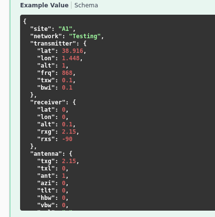
The first step to using the system efficiently is to setup a template. This is how we can save our settings for systems and reference them quickly for future calculations. Templates include information about the transmission and receiving station(s), such as heights, frequencies, power, antennas and environmental factors, some of which are discussed further below.
Making the Template
When designing a template for a C-UAS or RADAR system, we should apply additional consideration to the following:
Height Measurement
We can specify the height unit to be measured as Above Ground Level (AGL) or Above Sea Level (ASL), in either metres or feet. RADAR systems looking to locate fixed wing platforms are better suited for Feet ASL, whilst UAVs which use “GPS height” reference Metres AGL as their primary height reference, especially for restrictions which are also communicated as AGL. For example, consumer drones are restricted to 120m (400ft) AGL in the UK.
Running calculations in ASL is recommended for experienced users of CloudRF. When the transmitter location is changed, the height will need to be adjusted to consider the ground beneath. If not adjusted correctly, transmitters and receivers can be placed underground by accident resulting in an error.
Use AGL for UAV operations and ASL for high-altitude RADAR targets to match the domain/system altitude references.
Model
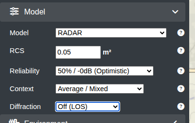
When designing a template for a RADAR system, the dedicated RADAR model should be used. This model is more that just line of sight as it uses a Radar Cross Section (RCS) value, allowing operators to define the size of targets they intend to detect where a drone has a smaller RCS (0.04) than a plane ( 6.0 ) which limits it’s detection range compared with a plane. By configuring appropriate RCS values, the model can more accurately represent real-world detection performance.
For a counter-UAS (C-UAS) system, the recommended model is ITU-R P.1812 with an average context, 50% reliability and diffraction turned off. This combination of model and diffraction will simulate the high frequencies and line-of-sight coverage utilised by C-UAS systems and has been proven to be the most accurate model during our model testing.
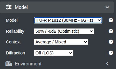
Use the RADAR model with RCS values of 0.05 for air-surveillance and ITU-R P.1812 (diffraction off) for UHF C-UAS sensors.
Environment
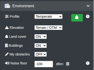
Obstacles affecting system coverage can be configured within CloudRF through the Environment submenu.
CloudRF provides access to extensive global clutter datasets, including 10m land cover, 2m building data, and, in selected regions, 2m LiDAR and tree canopy height data.
An interactive map showing the availability of this data can be accessed at the following link – https://api.cloudrf.com/API/terrain
SOOTHSAYERTM users can import their own LiDAR in addition to CloudRFs DEM archive.
For added accuracy, obstacle attenuation can be fine-tuned using clutter profiles, allowing operators to accurately represent real-world conditions. This level of customisation enables precise coverage predictions and improves confidence in system performance assessments especially at lower frequencies where NLOS attenuation needs to be considered as well as LOS.
To deal with temporary or new obstacles not currently in the DEM dataset, users can enable the ‘My Obstacles’ feature to manually draw or upload a KMZ/Geojson of the obstacle(s) to be included in the coverage prediction.
Noise
Noise is often an overlooked factor in radio network planning, yet its impact on coverage and performance is significant. By incorporating measured or simulated noise data, the planning environment will more accurately replicate real-world radio conditions.
This enables operators to reflect variations in the operating environment whether accounting for daily commuter traffic patterns or preparing for large-scale events such as concerts and sporting fixtures, where spectrum density and interference levels both increase substantially.
Noise is a factor within the template’s environment block. This value can either be manually entered eg. -100dBm or referenced from an uploaded dataset from multiple locations, creating a visible noise layer on the map.
Live noise can also be simulated in calculations by using networked SDRs. We have published an example capability here: https://github.com/Cloud-RF/DORA
Our recommended default settings are for Landcover and Buildings to be ON with the Temperate clutter profile which represents dense trees.
If you do not know the noise figure at your receiver, enter -100dBm which is typical of the ISM 2.4GHz band but will vary widely by location. Noise is measured across a channel so should be measured with the appropriate bandwidth. Johnson-Nyquist theory means (channel) noise increases with bandwidth and to a lesser extent, temperature.
| Bandwidth MHz | Channel Noise dBm |
| 1 | -114 |
| 10 | -104 |
| 20 | -101 |
Tools & Features
Once we have created a system template, we can use it with a number of tools to identify a transmission site and then determine the effective coverage from that location.
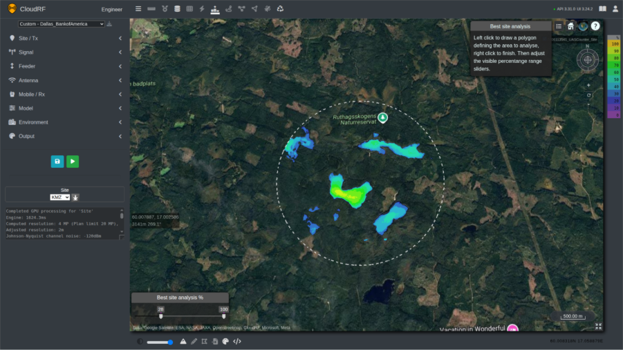
Best Site Analysis (BSA)
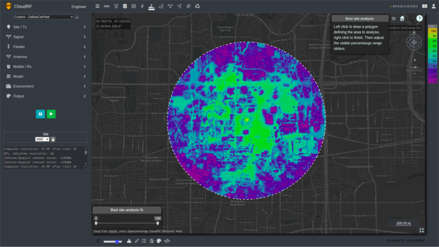
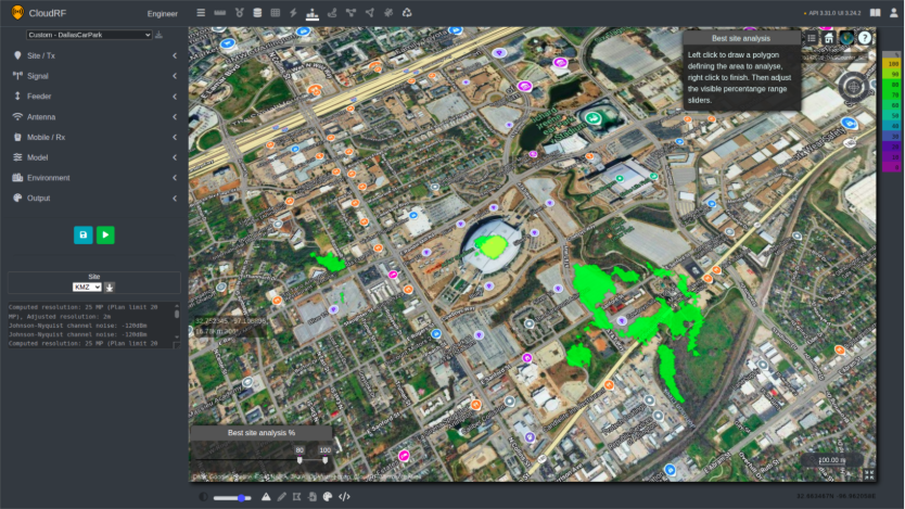
BSA is a powerful search tool designed to identify optimal transmitter placement locations defined by a geographical area. It performs hundreds of tests rapidly with a GPU in an area using a full propagation model with transmitter parameters. Positions are graded and then ranked to present the results as a heatmap image.
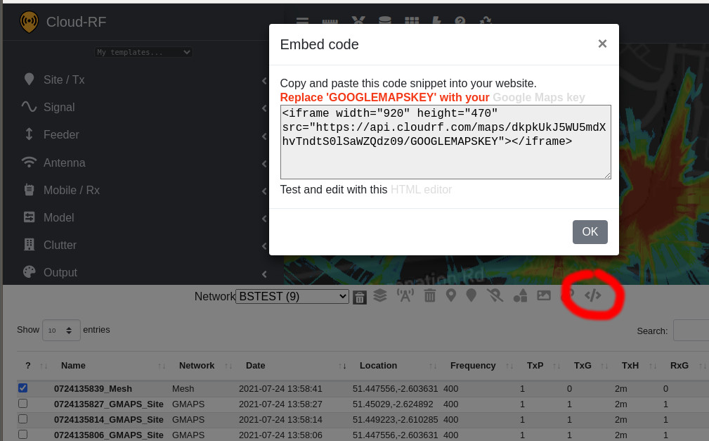
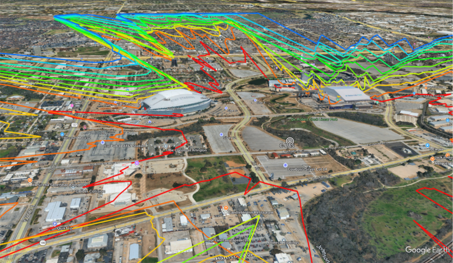
“The examples used in this document have been generated using KMZ and GeoJSON files. These can be imported into the User Interface (UI) via the Import Menu – Best Site Analysis. This is our recommended way to use the tool, as the simulation can be re-run with the same defined area and speed up the process when comparing a variety of height levels. There are numerous ways of doing this. Numerous software packages can do this; KMZ files can be created in Google Earth, and GeoJSON files can be created via geojson.io”
BSA is particularly valuable for identifying viable transmitter sites that may be overlooked through traditional planning methods such as “walking the ground” for example. By automating complex visibility analysis, users obtain actionable results within minutes, significantly reducing the time and effort associated with manual studies.
The recommended locations require interpretation. For example, if you are working with a DSM LiDAR model which contains water, this may be ranked as an efficient site. An operator will likely discount this, but that doesn’t mean that an adversary will as launching a drone from a boat is effective.
BSA ranks the most effective transmitter locations within an area using inter-visibility scoring.
Area Calculation
Once suitable candidate sites have been located, we can use the Area endpoint via the UI or API to see the coverage of our system at various heights. The heights chosen for the receiver will depend on the asset that we are looking to target with the C-UAS or radar system, for example 100m AGL.
The heatmaps created by the Area endpoint show the coverage of the transmitter to the receiver using the settings prescribed in the template. Heatmaps are useful for identifying areas with and without coverage and can assist in the decision-making process for the deployment of additional assets to further enhance coverage.
Area calculations can show coverage from a candidate site and expose gaps and shadowed airspace.
Best Server
Best Server is a feature which can be used with an established network. The Best Server tool will check each node for coverage to the designated receiver location. This allows the coverage from a large network of radios to be checked at various heights quickly, a common requirement when planning C-UAS, Radar or any Ground-To-Air transmission.
Best Server identifies which network nodes can affect a target at a given height and location.
Case Study 1 – C-UAS Site Selection – Texas, USA
Difficulty: Easy
This case study evaluates optimal C-UAS siting and coverage performance in the vicinity of a major sports stadium in Arlington, Texas.
Inputs
- C-UAS template
- Defined area of interest
Process
- Best Site Analysis to generate and score candidate locations
Outputs
- Coverage heatmaps per site (multi-height Area analysis)
- Identification of coverage gaps and shadowed regions
Decisions
- Select primary deployment site(s)
- Position additional systems for full airspace coverage
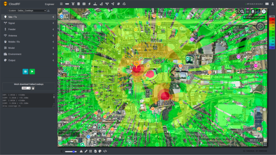
The system represented by the template in this simulation is an omnidirectional C-UAS system, operating at 2.4GHz, with a 3m tall antenna. For the initial survey, the receiver height is set to 150m AGL, this can be reduced for more in-depth planning throughout the planning process.
The model used for this survey is ITU-R P.1812, with diffraction turned off. Within the city of Arlington, there is 2m LiDAR available, which has been selected by setting the Environment to Surface/DSM (LiDAR), and a resolution of 2m.
With the template for the C-UAS created, Best Site Analysis can now be used to identify optimal locations for siting the system.
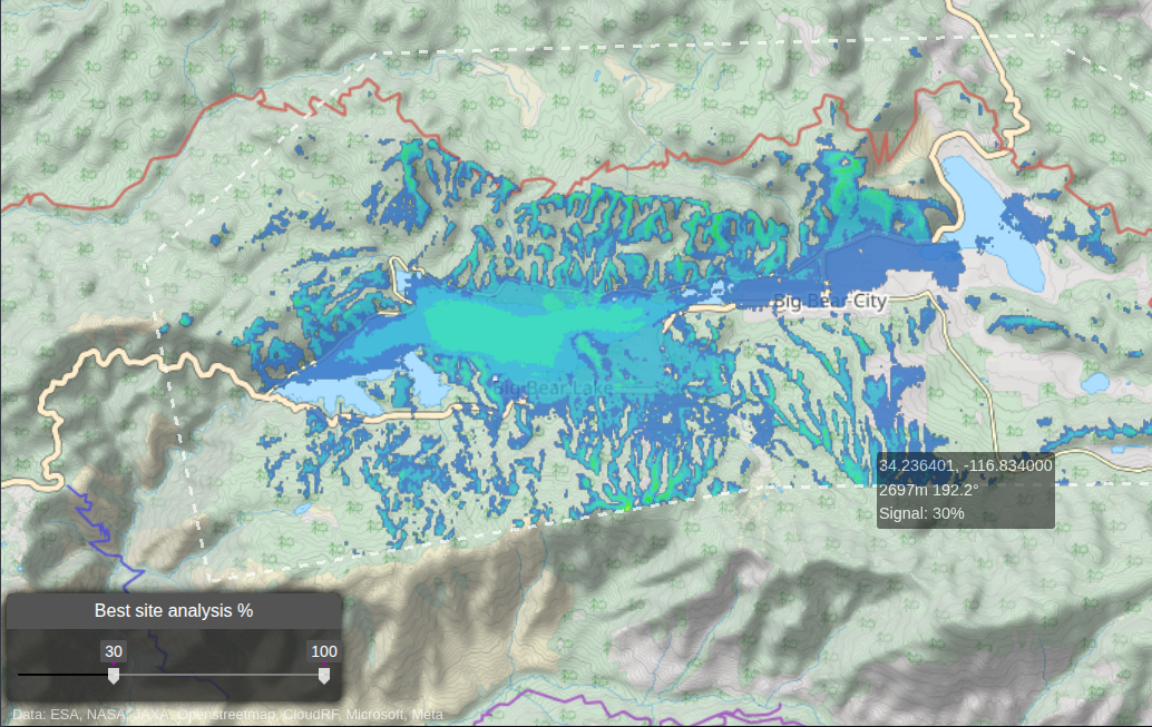
After defining the desired area of coverage, we are presented with a layer with sites scored according to their intervisibility.
Using the slider to filter out lower-scoring positions, areas with higher intervisibility can be highlighted on the map.
Based on the analysis, the highest-scoring sites were located on the roof of the stadium and towards the car parks on the South side of the stadium.
“For best practice, we recommend evaluating numerous positions. In the above example, the centre of the stadium is the optimal position. However, it is not in a practical sense, i.e. is the stadium roof safe? Other considerations could include access rights, sustainment and logistical requirements.”
With these positions identified, the Area endpoint can be used to evaluate the coverage.
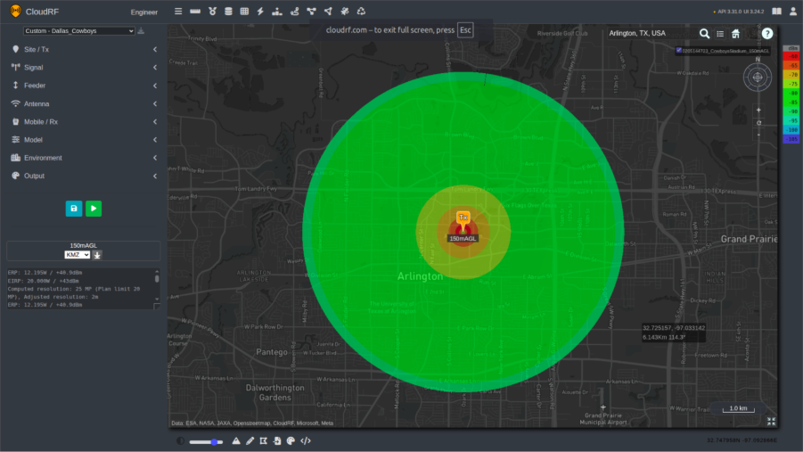
Setting the receiver at a height of 150m AGL, there is good coverage within a 5km radius of the transmitter. The weakest areas of coverage are directly overhead of the transmitter, where the null of the dipole has the lowest gain.
UAVs can operate at different heights so coverage should be evaluated at a variety of receiver heights within the local threat capability. For the next simulation, the height of the receiver is set to 10m AGL.
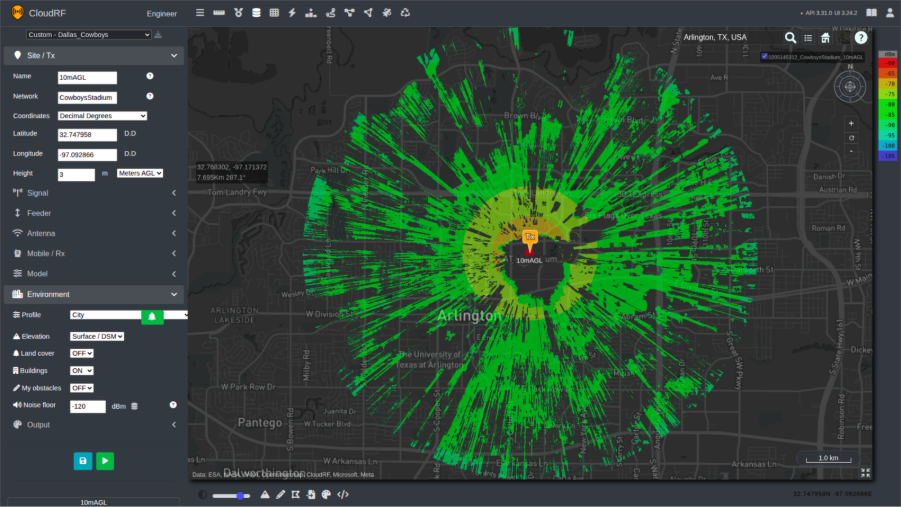
The coverage of the C-UAS system is now reduced. Obstacles in the environment, including buildings and trees, have a greater effect on the signal, blocking the line of sight and reducing overall coverage.
A particular point of focus is the area directly around the transmitter. Due to the curvature of the roof and the relative height of the building compared to the ground, positioning the C-UAS system on the roof creates shadows around 400m away from the stadium, where there is no coverage.
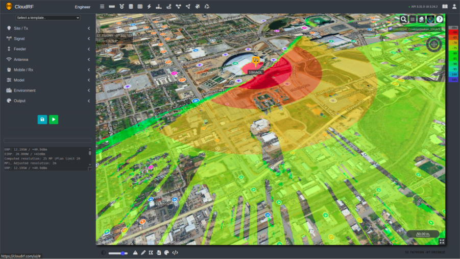
One chain of thought for solving this issue could be to position the transmitter on the side of the stadium. By changing position and re-running the simulation, there is an improvement in coverage to the South of the stadium, but now the stadium is blocking a large majority of the signal to the North, requiring the deployment of further systems to provide coverage in the area required.
Having multiple sensors improves system resilience to failure or interference and improves detection.
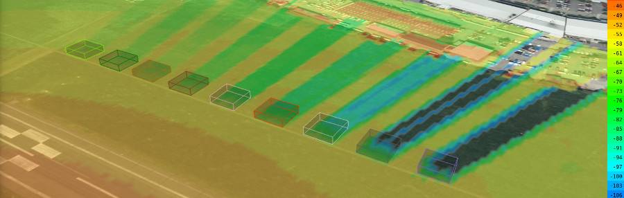
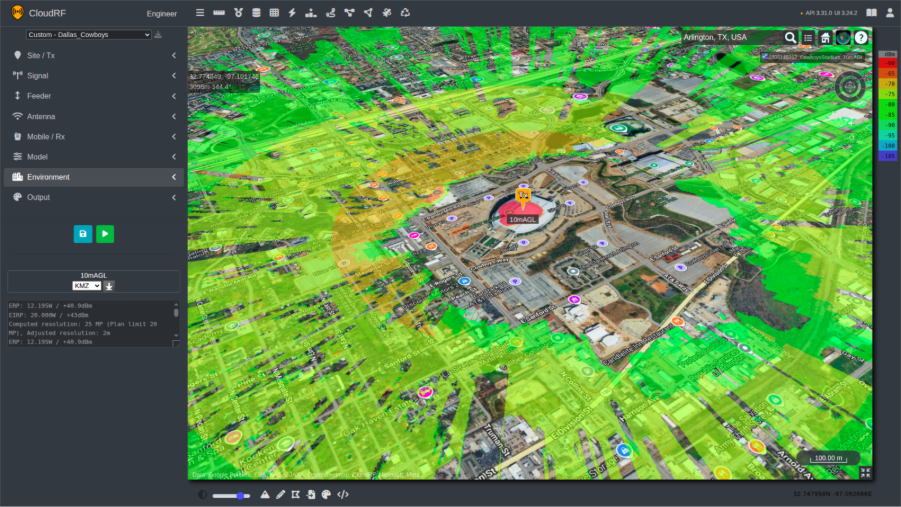
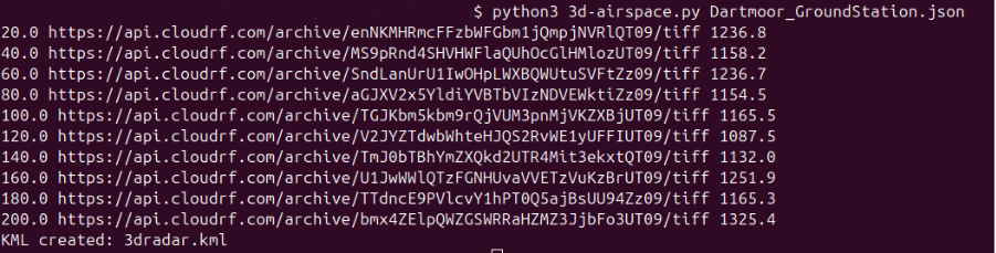
Alternate locations identified during the initial Best Site Analysis can also be assessed for deployment of the C-UAS system. For example, positioning the transmitter in the car park to the south of the stadium allows us to save a site template and quickly generate 3D airspace coverage using the 3D-Airspace script. This enables rapid visualisation of coverage performance at multiple altitudes.
This script will create a KMZ showing multiple layers based on the height of the receiver. In this case, with an upper ceiling of 150m, the script will create layers every fifteen meters.
The script using these requests is available via https://github.com/Cloud-RF/CloudRF-API-clients/tree/master/python/3d-airspace.
From this analysis, there is greater coverage of the southern side of the stadium, previously in the shadow of the C-UAS site on the rooftop. The stadium itself is still acting as a major obstacle; the deployment of multiple systems would be required to cover the entire stadium area.
Adding multiple systems into this network and creating a single layer to demonstrate coverage is possible by using the Superlayer tool, allowing commanders and operators to get a clear overview of sensor coverage.
The Best Server tool can also be used to evaluate a network of C-UAS systems. Using the established network, a UAV can then be added into the simulation, flying at a height of 25m in the example below. This can then show us which C-UAS would be able to have an effect on the UAV. In the example below, the UAV at 25m AGL has a link to the C-UAS systems in the northern area, whilst the systems deployed on the rooftop and in the southern car park are being blocked by obstacles.
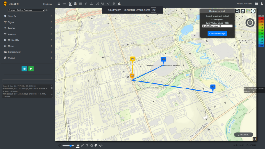
BSA identifies viable deployment positions, and multi-height Area analysis shows where additional systems are required for full stadium coverage. Best Server can be used to quickly identify coverage from selected positions to a central receiver.
Case Study 2 – Finding the Operator – Dartmoor, UK
Difficulty: Moderate
CloudRF can be used for simulating both transmitters and receivers in a real-world environment. In this case study the template and tools used will show how the simulation results can be interpreted to understand where the ground control station (GCS) could possibly be located.
Inputs
- DF sensor template
- Sensor height and frequency
- Line of Bearing (LOB)
- Measured received power
Process
- Path-loss calculation using DF-derived constraints
Outputs
- Probable GCS transmitter locations
- dB error score per location
Decisions
- Prioritise ground search locations
- Assess the control range of the UAV
DF sensors are essential for a C-UAS team in order to locate both the UAV and the corresponding control station. These systems can come in a variety of formats and may use various methods to determine a Line Of Bearing (LOB) to the transmitter.
Direction Finding (DF) sensors are typically deployed in multiples to generate several Lines of Bearing (LOBs), enabling triangulation and the establishment of a Position Fix (PF) at the point of intersection. However, this represents an ideal scenario. In practice, operational constraints such as logistics, network limitations, and manpower availability may restrict deployment to a single asset, significantly reducing geo-location accuracy.
In the following example, CloudRF’s API is being used to help a C-UAS team with a single DF system to identify possible locations of a UAS ground control station (GCS).
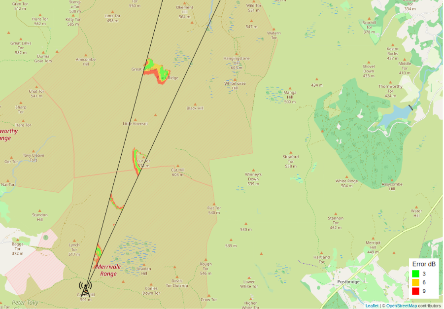
The methodology for doing this is not dissimilar from the standard way of using the software, with the user creating a template for the asset they are looking to locate. For this example, the height of the DF system was set to 8m, and the ground control station was set to 2m. Measured units are changed to Path Loss which shows possible signal coverage irrespective of power levels and is recommended when working with unknown power levels or receivers.
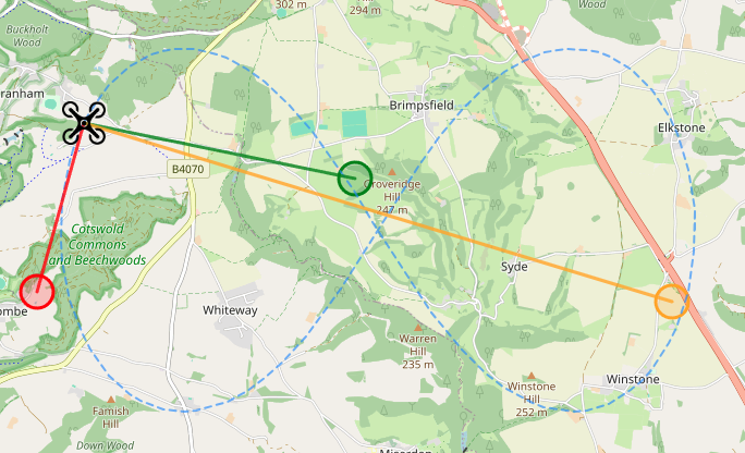
By filtering the results of this simulation through parameters collected by the DF system, such as the LOB and received power of the signal, possible transmit sites can be identified on the map, scored with colours representing error in dB.
This result can provide operators with a greater understanding of where a rogue transmitter could be located with just one DF system, increasing the efficiency of a single team. For more on this concept see our DF blog.
In the screenshot below, a single LOB has been used to evaluate a large area to determine several possible sites. False positives in nearby dead ground are expected which can be quickly discounted using other sources of information.
Once a location has been identified, operators can use the Area endpoint to evaluate the coverage of this transmitter to determine the threat range of the UAS. This can be done within the UI as demonstrated in the screenshot below.
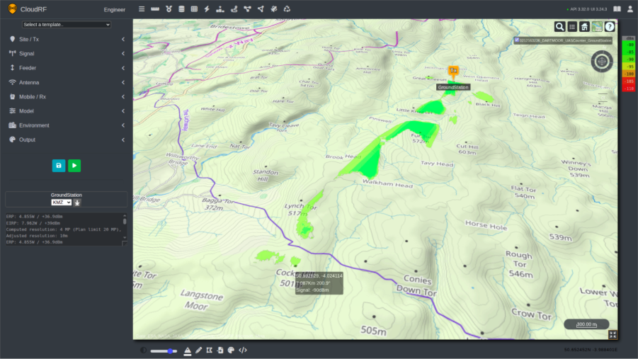
For evaluating the coverage of the ground station at various altitudes, a 3d-airspace script can be used to recursively model coverage efficiently at ascending heights.
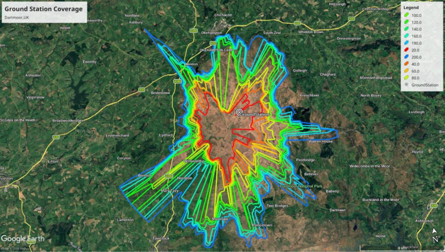
A single DF sensor combined with path-loss modelling significantly reduces a large search area.
Integrating AI
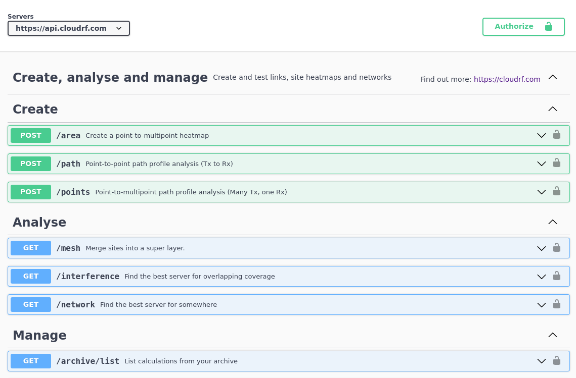
An open architecture with published documentation and examples enables Large Language Models (LLMs) to quickly build custom interfaces and tools to leverage the Open API.
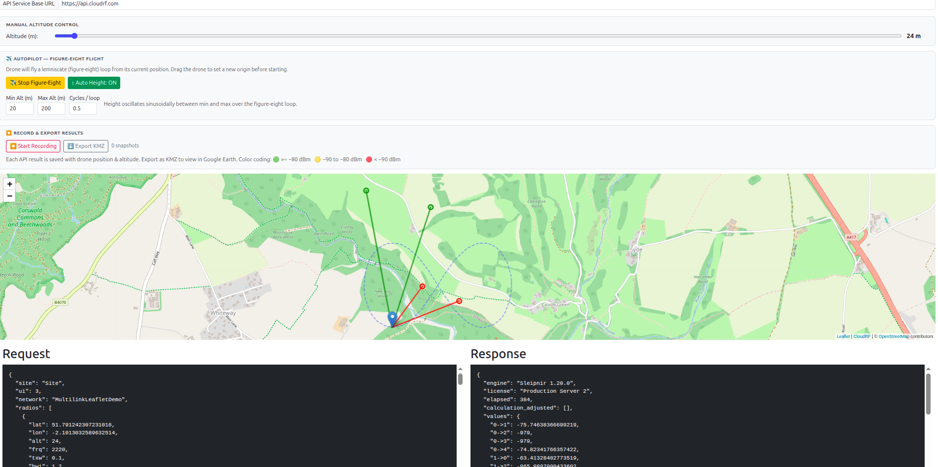
Here is an example sensor placement interface built with Claude, which exploits the new Multilink API to show coverage for a UAS. The tool uses pre-defined templates, so it requires no RF engineering skill or training to move the sensors to achieve coverage with high confidence.
Live demo link: https://cloud-rf.github.io/CloudRF-API-clients/slippy-maps/leaflet-drone-detection.html
Conclusion
Pre-deployment planning for C-UAS and RADAR systems is resource intensive and traditionally required expert input.
By standardising system parameters in reusable templates and using efficient analysis tools powered by open APIs, modern operators can model entire networks quickly and accurately without compromising quality.
Optimal locations are not always the most obvious or the most practical. A single system rarely provides complete protection in complex environments so a layered, networked approach, validated through high resolution simulation, enables continuous airspace coverage and ensures that assets are positioned for maximum effect.