We’ve published a series of video tutorials for HF novices to bring to life HF theory around the topics of Frequency selection, Antenna fundamentals and forecasting.
HF communications is very different to terrestrial communications and given the right frequency, time of day, and antenna, you can achieve long range links in excess of 1000km with only a few watts of power on a HF Dipole.
CloudRF’s API uses the proven VOACAP engine to create accurate HF predictions considering a number of factors. Using this tool, you can plan long range resilient links and anticipate the (time based) surprises HF throws up…
Frequency Selection
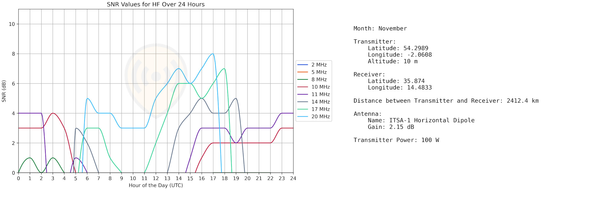
Time is critical to HF communications. As sunlight changes throughout the day, so does the range of usable frequencies. A common strategy for round the clock communications is to maintain a day and night frequency. These can be identified using the VOACAP powered path tool in CloudRF.
This tool reports the Signal-to-Noise ratio against time for different HF frequencies.
Antenna Basics
Once a frequency has been identified, an antenna must be constructed to the right dimensions.
The antenna of choice for many long range HF links is the half wave dipole. This simple and efficient design uses two fixed length elements and a center feeder to bounce signals off the ionosphere.
To get the wavelength for your frequency divide 300 by the frequency in MHz.
Height
The height of the antenna will change its radiation pattern and the take off angle.
Achieving at least a quarter wavelength is recommended for efficiency (and practicality) as the long HF wavelengths make a half wavelength too high for most masts. For an 11MHz signal, the height would need to be 6.8m for example.
Azimuth
HF patterns are directional and must be orientated towards a distant station. For some antennas, like long end fed wires this is as simple as pointing the wire towards the station.
For a half wave dipole, which has a donut shaped radiation pattern, it must be broadside towards the station as it has nulls where the wire ends are. A bad azimuth can be forgiven at short range but will determine the potential range.
Feeder loss
Using a feeder co-axial cable will reduce the efficiency of your system. The effect increases with length so you should aim for the shortest, low loss, feeder possible. The impact of the feeder can be simulated even if you don’t know the cable type by entering 1 or 2dB into the feeder loss option.
Forecasting
Sunspot R12
The Sunspot index number describes solar activity which follows a 10 year cycle. When the number is high, there is increased solar activity and better refraction. The different between a good and bad year within the cycle is around 6dB which on the S Meter scale is equivalent to two levels, or the difference between success and failure.
This can be predicted and the random element budgeted for using the model’s reliability value.
