Simulating radio coverage shows where a signal can reach, but to see how fast a data signal could be, we need to measure its throughput.
Throughput is a key performance requirement for digital radio systems and determines what a link is capable of. By simulating a link’s throughput, planners can confidently establish high throughput, spectrum efficient, links which can support high data rates and avoid last minute fixes such as increasing the power.
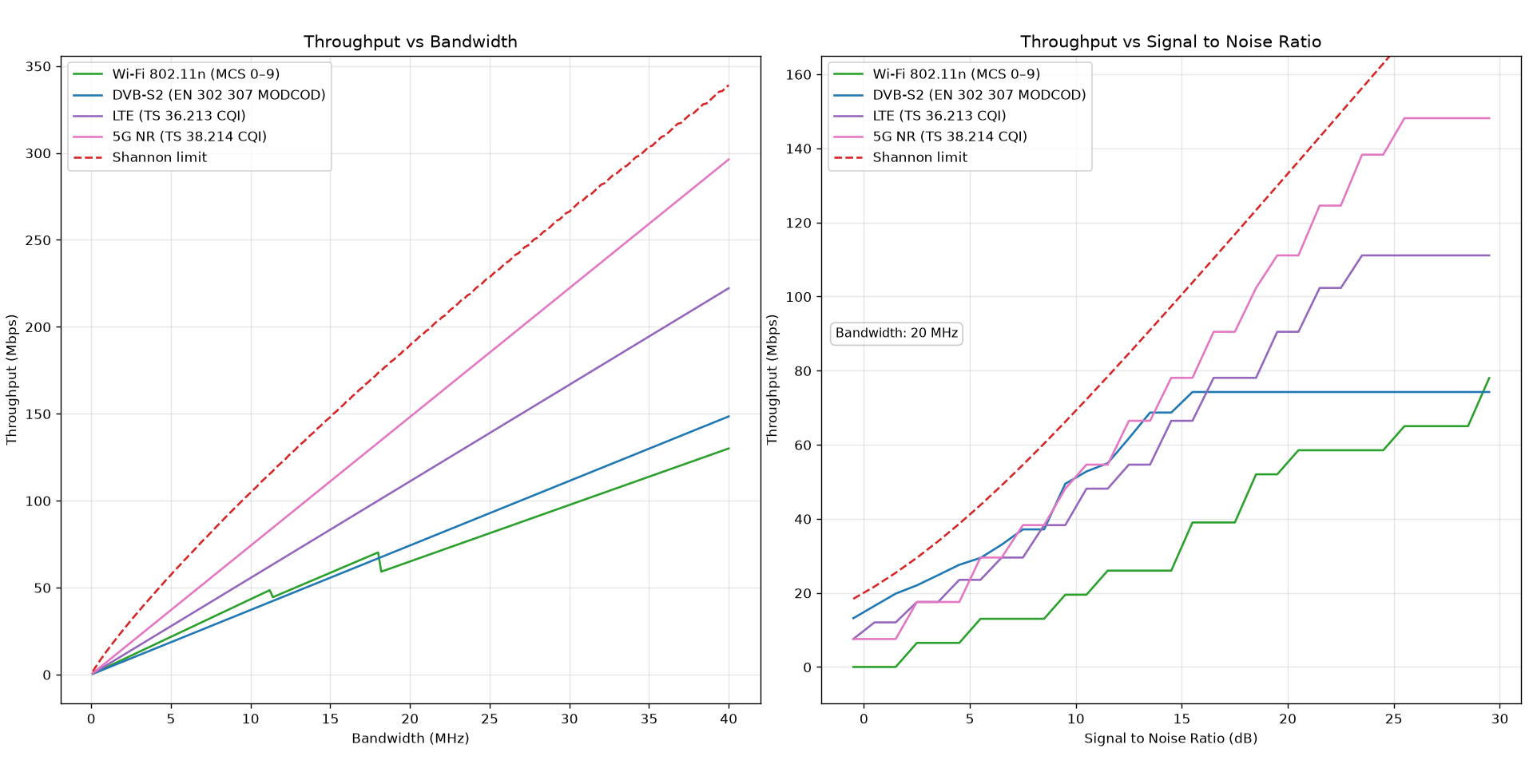
Throughput at different channel bandwidths
Throughput theory
Within the context of digital signal processing, throughput is the amount of data, measured as bits, that can pass through the network or link within one second (Bits-Per-Second).
It is a popular metric that all radio users can benefit from, even if they don’t understand it directly. For instance, a consumer could use throughput to choose an internet service provider for their home network, whilst a video broadcasting manager may site their infrastructure in order to provide smooth high-definition video.
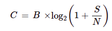
The most famous method for calculating throughput is the Shannon-Hartley theorem, which determines the maximum data rate or channel capacity, that a communication channel can carry, based on several variables:
C = Channel Capacity, in bits per second.
B = Bandwidth, in Hz.
S/N = Signal-to-Noise Ratio (SNR), expressed as a power ratio.
Bandwidth
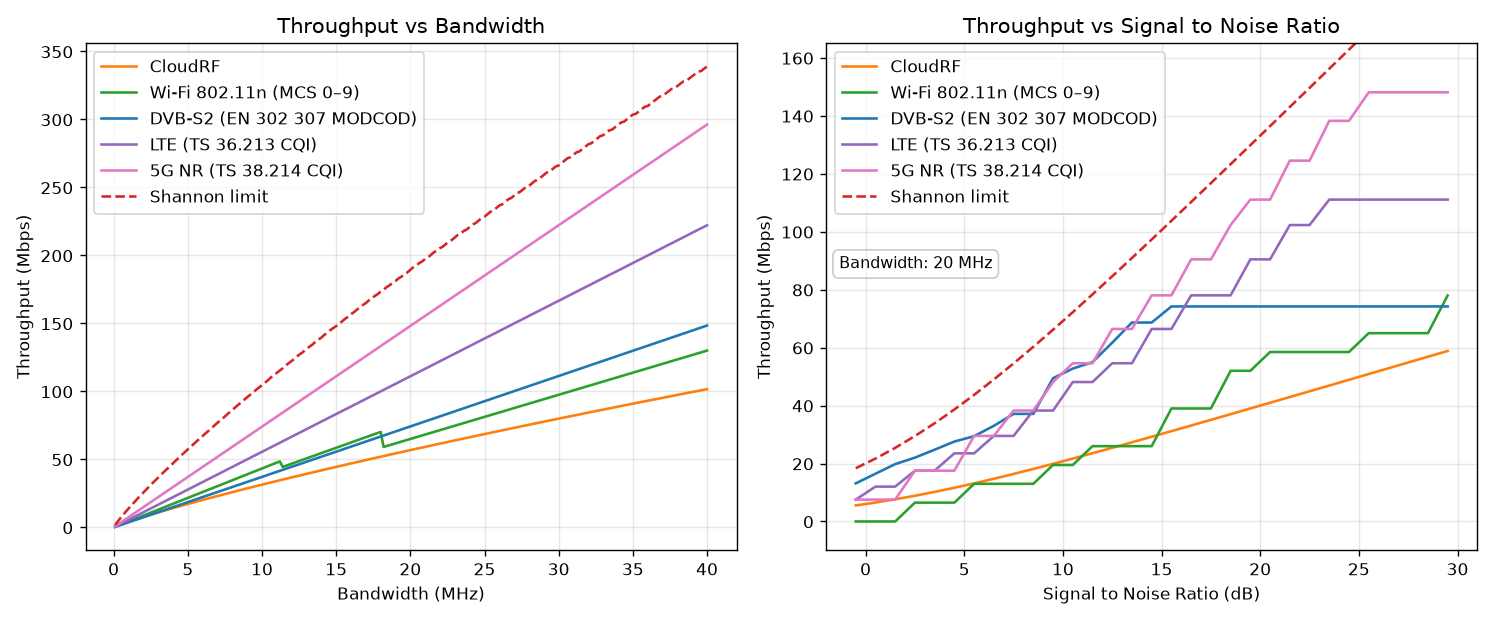
Bandwidth is the frequency range that a channel occupies. It defines how much raw capacity is available before signal quality is considered. When comparing the relationship between bandwidth and channel capacity in a mathematical sense, bandwidth scales channel capacity linearly so doubling the bandwidth doubles the channel capacity under ideal conditions.
Increasing bandwidth also increases thermal noise because a wideband receiver will receive more adjacent radiation, as determined by Johnson-Nyquist noise. Bigger is not always better.
The relationship between bandwidth and channel capacity can be illustrated by comparing technologies such as HF and 5G NR, which sit at opposite ends of the bandwidth spectrum. A typical HF channel occupies around 3KHz of spectrum while a 5G NR channel can be 100MHz. Comparing the throughput of both channels with a consistent 30dB SNR, the HF channel provides a capacity of around 30Kbps, whilst the 5G channel could provide close to 1Gb/s
Signal To Noise Ratio
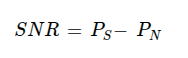
Signal-To-Noise-Ratio (SNR) is a Key Performance Metric (KPI) used to measure signal quality and is calculated as a basic ratio in decibels:
SNR = Signal-to-Noise Ratio.
PS = Signal power in dBm.
PN = Noise power in dBm.
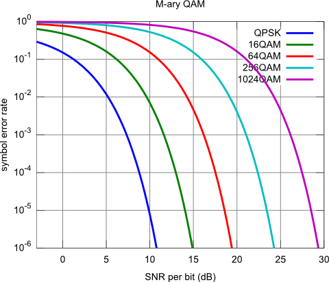
As SNR rises, a receiver can reliably decode denser, more efficient modulation schemes like QAM, and as it falls, getting closer to and surpassing the noise floor, the modulation must fall back to simpler, more robust methods like BPSK.
This effect is most commonly seen with mobile phones. When a phone has a full signal, it can stream high quality video using a high modulation rate and when it has a weak signal it can only just send a text message.
Channel capacity doesn’t take into account the modulation scheme or waveform which will ultimately determine the information rate. Most waveforms employ error correction which will provide resilience at the expense of speed.
For reference, we can use the following table for SNR requirements:
Modulation
Required SNR (dB) at 10–2 bit error
Application
BPSK
2
GPS / Telemetry
QPSK
5
Telemetry / Text
16-QAM
9
Low quality video
64-QAM
14
Medium video
256-QAM
18
High quality video
The relationship between SNR and modulation is established in radio systems through Modulation Coding Scheme (MCS) index tables. Each MCS index corresponds to a modulation type and coding rate with a minimum required SNR. Lower MCS indexes use slow and robust schemes such as QPSK, which tolerates a noisy environment or weak signal.
The Bit Error Rate increases with noise so to maintain functional communications, the schema must ‘step down’ as a channel deteriorates at the cost of speed. This is why your phone gets slower the further away you go from the tower.
Higher MCS indexes can use dense modulation schemes like QAM-64, carrying 6 bits per symbol (26 = 64), but are only usable while SNR is high enough to avoid excessive bit errors. So for systems using MCS indexes, we can see that throughput increases in steps, with each step corresponding to a waveform.
Simulating Throughput….for anything
CloudRF is technology agnostic by design, supporting a wide variety of diverse communications systems from HF to 5G NR, all bound by physics not marketing departments.
For this reason, CloudRF’s throughput simulation has been designed to be conservative relative to both the channel capacity and common MCS indexes. It is aligned with the 802.11 MCS index, designed around wideband 20/40MHz channels.
The Shannon-Hartley theorem represents the theoretical ceiling of throughput, not the realistic levels of what even high data-oriented technologies can achieve in the field. There are numerous factors that affect both the bandwidth and SNR of a signal which will limit the throughput. A conservative estimate is therefore an honest reflection of what operators can achieve and if simulation inputs are accurate, it is a modest estimate.
In our experience of setting safe defaults for busy users, going conservative early is a safe strategy as users will be able to plan sites which go on to exceed their expectations whilst avoiding sites which may disappoint.
There is also the question of accessibility. CloudRF is used by a wide spectrum of users, from experienced RF engineers to occasional or first-time radio users who may not have a working knowledge of modulation and coding schemes. Precisely modelling throughput by technology (LTE, 5G NR etc) would raise the barrier to entry and increase the risk of error and cost of training.
By using a conservative, technology-agnostic estimate, CloudRF gives casual users a reliable, usable figure for radio planning today.
Video demo: Wi-Fi coverage at a holiday site
Outdoor WiFi throughput simulation
Example: Throughput at a large festival
For this example, we’re going to model throughput for a system at the Glastonbury Festival in the UK. This significant event attracts over 200,000 people in a dense rural area, competing for limited spectrum.
A physical survey may identify areas of no coverage due to the topography of the land and clutter like vegetation, but it can’t predict how temporary obstacles which aren’t represented will affect coverage. Likewise, the future interference from new transmitters, and crowds, in the area cannot be taken into account.
Therefore, for events such as these, we can use planning software to evaluate coverage and identify optimal sites and settings.
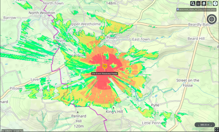
The heatmap below is derived using the equipment’s receiver sensitivity based on Received Power (dBm). When looking at coverage using this unit, variables such as noise and bandwidth are not taken into account. This can be useful for a quiet environment and for evaluating the coverage range, but this ideal prediction will not represent the environment during the event…
Received Power with DTM and Landcover
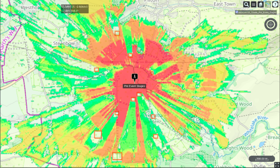
The first challenge is the issue of temporary structures, which are currently not present. By using DIY clutter, temporary obstacles can be included in our modelling. This includes setting the height and attenuation in order to accurately represent the materials. In this example, the future obstacles have reduced coverage, creating notable gaps.
Received Power with DTM, Landcover and custom clutter
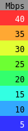
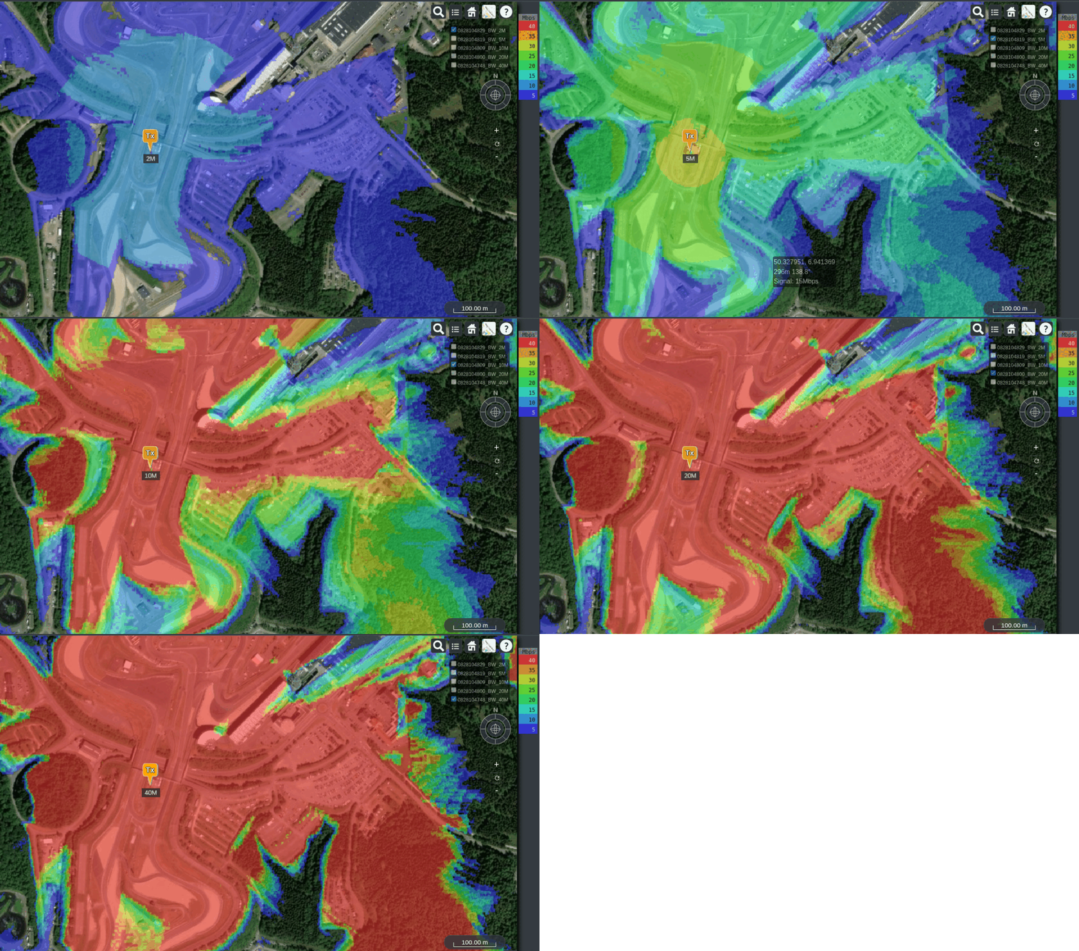
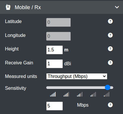
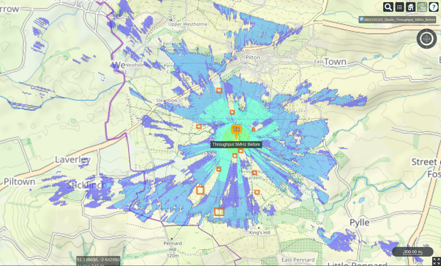
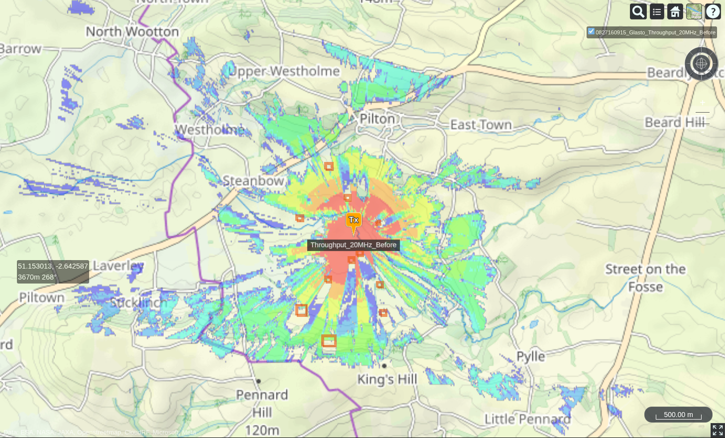
With our overall coverage determined, we can now move on to looking at the throughput (Mbps) by setting the channel bandwidth and the estimated noise affecting our signal. For this example, bandwidth increases from 5MHz to 20MHz, with thermal noise increasing accordingly from -107dBm to -101dBm. The colour threshold was set at 5Mbps.
Throughput for a 5MHz wide signal
Throughput for a 20MHz wide signal
By comparing the two bandwidths, we can see that, in optimum conditions, the larger bandwidth is achieving a greater throughput while the coverage for the lower bandwidth channel is slightly better.
The next step in simulating our event is to budget for local noise. Noise values can be sourced from spectrum analysers or cognitive radios and will normally provide a better local reference for planning than thermal noise although be aware that some measure noise differently. For this example, we are using an elevated noise figure for the channel which was recorded at at the previous years festival.
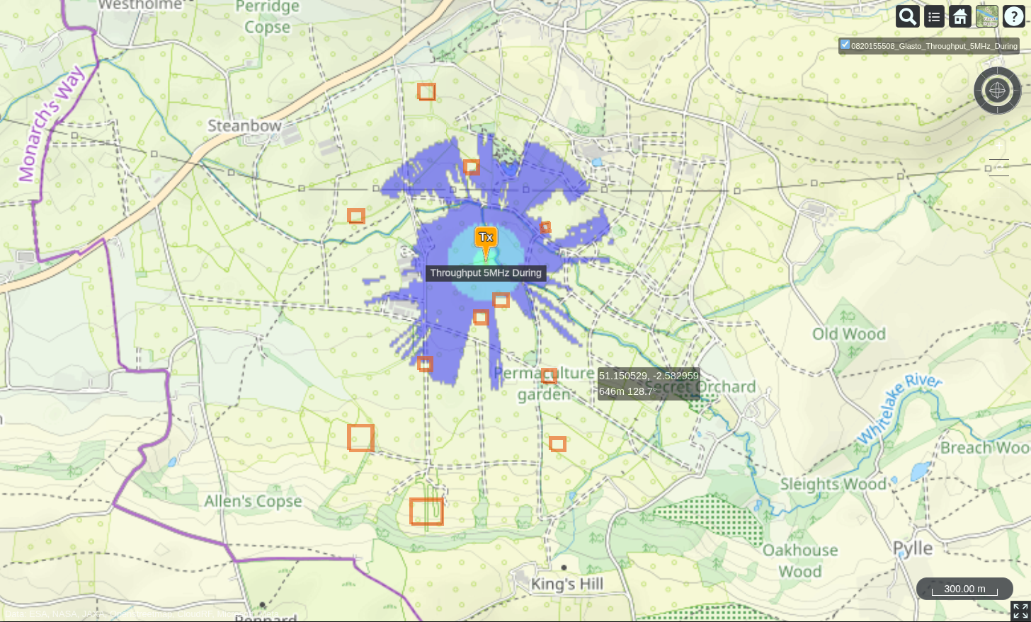
Throughput for a 5MHz signal with very high local noise
With a bandwidth of 5MHz and the noise floor significantly raised at -85dBm, the simulated throughput is significantly reduced compared to the thermal noise floor prediction. This represents a worst case scenario.
Regardless of which channel option is chosen, by conducting a planning process, planners can visualise the network’s potential during both quiet and noisy conditions and plan accordingly.
This website uses cookies to improve your experience while you navigate through the website. Out of these, the cookies that are categorized as necessary are stored on your browser as they are essential for the working of basic functionalities of the website. We also use third-party cookies that help us analyze and understand how you use this website. These cookies will be stored in your browser only with your consent. You also have the option to opt-out of these cookies. But opting out of some of these cookies may affect your browsing experience.
Necessary cookies are absolutely essential for the website to function properly. This category only includes cookies that ensures basic functionalities and security features of the website. These cookies do not store any personal information.
Any cookies that may not be particularly necessary for the website to function and is used specifically to collect user personal data via analytics, ads, other embedded contents are termed as non-necessary cookies. It is mandatory to procure user consent prior to running these cookies on your website.