When simulating radio propagation you can choose to model results in a variety of ways: Path loss will show you the attenuation in decibels (dB), Received Power will show you the signal strength at the receiver in dBm and field strength will show you the signal strength in micro-volts (dBuV/m). If you are using a digital modulation schema such as Quadrature-Amplitude-Modulation (QAM) your effective coverage will be dictated by the desired Bit Error Rate (BER) and local noise floor. This blog will describe these concepts and show you how to apply them to model a given modulation schema.
Bit Error Rate (BER)
The Bit Error Rate (BER) is the number of acceptable errors you are prepared to tolerate. This is typically a number between 0.1 (every 10th bit is bad!) and 0.000001 (Only one in a million is bad). This ratio is closely linked to the Signal-to-Noise-Ratio (SNR) which is measured in decibels (dB).
A high SNR is required for a low BER. A low SNR will have an increased BER. Put simply a strong signal is better than a weak one and has less chance of errors.
The reason error increases with SNR is because of noise. The closer you get to the
noise floor for your band (about -100dBm at 2.4GHz), the more unstable and unpredictable things become.
| Decimal | Exponential | Link quality
|
|---|
| 0.1 | 10e-1 | Bad
|
| 0.01 | 10e-2 | Not bad
|
| 0.001 | 10e-3 | OK
|
| 0.0001 | 10e-4 | Good
|
| 0.00001 | 10e-5 | Very good
|
| 0.000001 | 10e-6 | Excellent
|
The noise floor
The noise floor is the ambient power present in the RF spectrum for your location, frequency, temperature and bandwidth. Understanding the noise floor is important when modelling Bit Error Rate as it is subject to change and will determine your SNR. The SNR will determine your BER so if you want good coverage you need to know your noise floor so you can set your power accordingly. There are several factors that influence noise floor:
Location
A lot of noise if man-made so the noise floor is higher in a city than in the mountains. The difference varies not just by city but by country as countries have different spectrum authorities and regulate spectrum usage differently. The difference between a city and the countryside for a popular band like 2.4GHz is huge and can be over 6dB. Using a calibrated spectrum analyser with averaging is a good way to measure the noise floor. Ensure you set the bandwidth to your system’s bandwidth for best results.
If you don’t own a spectrum analyser you can use
Boltzmann’s Constant (see bandwidth section) and add an arbitrary margin to it depending on your location. This table has some suggested generic values:
| Location | Signal | Noise floor
|
|---|
| Rural / Remote | WiFi 2.4GHz | -101dBm
|
| Suburban | WiFi 2.4GHz | -98dBm
|
| Urban city | WiFi 2.4GHz | -95dBm
|
| Rural / Remote | WiFi 5.8GHz | -98dBm
|
| Suburban | WiFi 5.8GHz | -95dBm
|
| Urban city | WiFi 5.8GHz | -92dBm
|
Frequency
Thermal noise is spread uniformly over the entire frequency spectrum but man-made noise is not. The 2.4GHz ISM band is much busier than neighbouring bands for example due to its unlicensed nature. As a result the noise floor is several dB higher than a ‘quieter’ piece of the RF spectrum. Some of the quietest spectrum is co-incidentally the most tightly regulated, which keeps users down, which reduces noise, and improves performance.
Temperature
Thermal noise increases with temperature so in general you will get
slightly more distance for your power in northern Scandanavia than in central Africa. The difference is about 1dB between a cold day and a hot day so can be considered negligible when compared with other factors. Budget for a hot day with an extra dB in your planning.
Bandwidth
Bandwidth has a direct influence on noise power because of Boltzmann’s Constant. This simple formula lets you calculate the absolute noise from the bandwidth. There are different ways to apply the formula but if you use dBm then the simplest form is:
Noise floor dBm = -114dBm + 10 Log(Bandwidth in MHz)
Using this formula you get the following results.
| Receiver Bandwidth MHz | Noise floor | Equivalent system
|
|---|
| 0.1 | -124dBm | LPWAN
|
| 1.0 | -114dBm | Bluetooth
|
| 10 | -104dBm | WiFi 10MHz
|
| 20 | -101dBm | WiFi 20MHz
|
| 40 | -98dBm | WiFi 40MHz
|
| 100 | -94dBm | Spectrum analyser with 100MHz FFT
|
If in doubt, use a noise floor of -98dBm
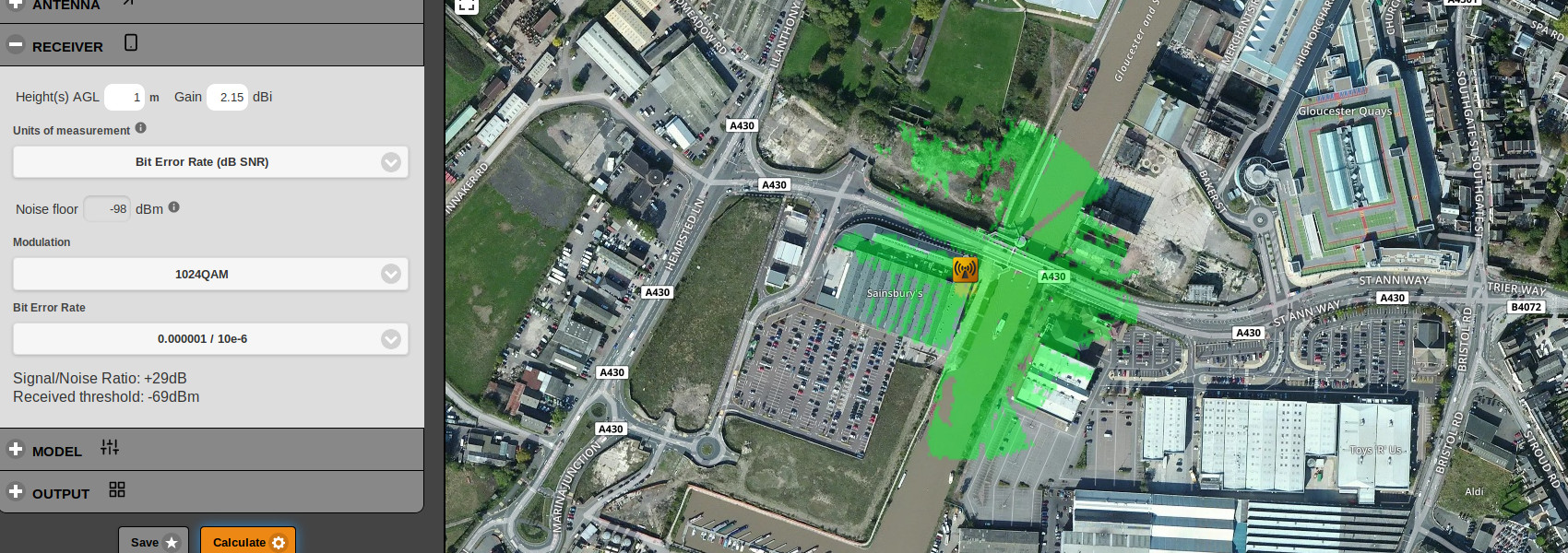
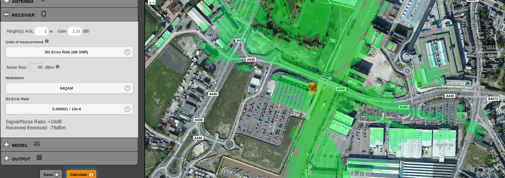
Example
A low power 20MHz wide 64QAM signal is being simulated in a city. The noise power is computed from the bandwidth with Boltzmann’s Constant as -101dBm to which we add +3dB for man-made noise putting the
noise floor at -98dBm.
When selecting a BER of 0.1 / 10e-1 the SNR is 11dB which equates to a receiver threshold of -87dBm.
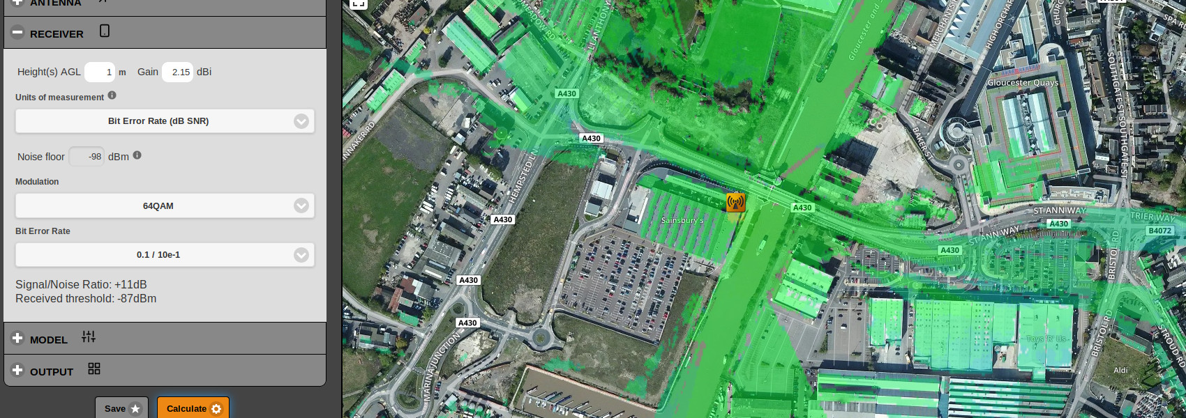
The difference in propagation between the two error rates is noticeable with 64QAM but what happens if you switch up the modulation to 1024QAM which carries a higher SNR?