To Survey or Simulate

Whether its survey drones, drive test vehicles or a police analyst with a backpack full of phones, the problem is the same: RF propagation surveys are very resource intensive. They’re more accurate than a simulation, but not more efficient.

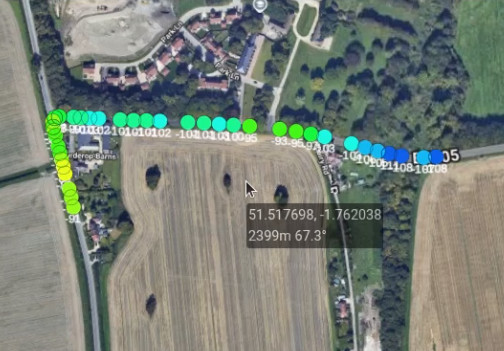
Survey data is typically a GPS log with signal metadata including a signal strength value. This can be different measurement units but the principle is the same. It is data which shows the signal at a given point.

Surveying is preferred for good reason by some industries, especially for evidential purposes where the variables in simulation open the door to uncertainty which nobody wants in court. Another reason is legacy desktop simulation software is slow and often inaccurate, especially amongst clutter which is more complex than a topographical study.

For example, relying upon a high-low empirical model like Hata which pre-dates developments in clutter will get you ~8dB accuracy whilst calibrated survey equipment can get you ~2dB, or ~3dB for an app on a standard phone.

Manual calibration

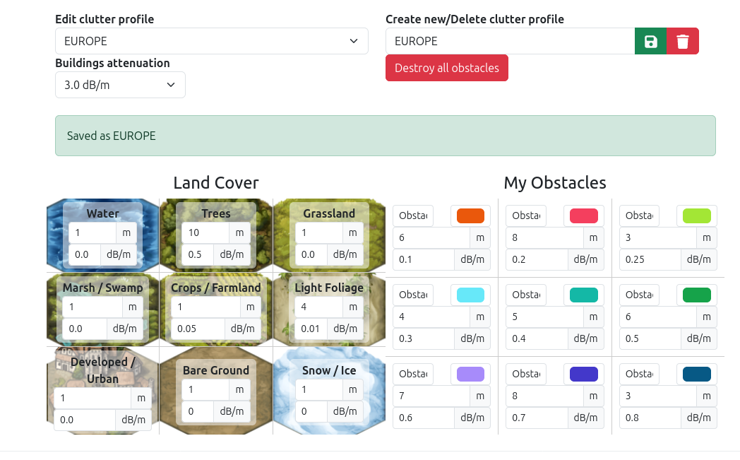
Using survey data like the output of Rantcell’s survey app, we can load this into our web interface to perform calibration manually. This process involves adjusting model and/or clutter settings until the error between the simulation and the measurements is as low as possible. It’s an efficient process as you can test thousands of points in a single API call but also repetitive, interface based and requires engineer input to adjust clutter values for example. You can see manual calibration in action here.

A good calibration would be below 8dB. For more on calibration of survey data, see one of our many field test blogs.

Good survey data is thousands of points all around a site of interest. When we’re field testing, we choose our route to ensure we collect a diverse range of data.

The Pizza Problem

The pizza problem is when you only have a slice of data but need to infer the rest. This is very common in the real world where a customer may not be able to collect data all around a site for various reasons:

• Lack of time
• Lack of access
• Lack of resource

This limited data is then used to estimate what the rest of the coverage looks like. For an omni-directional antenna, it’s a good assumption. For a directional antenna, it’s clearly less accurate but crucially, it is about making the best estimate using available data.

If you can get more measurements, then do it. If you don’t have the time/resource, then simulation using calibration offers the best compromise. After all a ~7dB accuracy prediction is much more useful than no coverage at all.

A Machine Learning genetic algorithm

Using a slice of data, we can employ a basic Machine Learning model which uses a genetic algorithm to optimise settings. It works by starting with a range of fixed inputs (tower frequency, location etc) and a range of variables (power, tree height, building thickness etc) which it uses to make pseudo-random requests to our Area API.

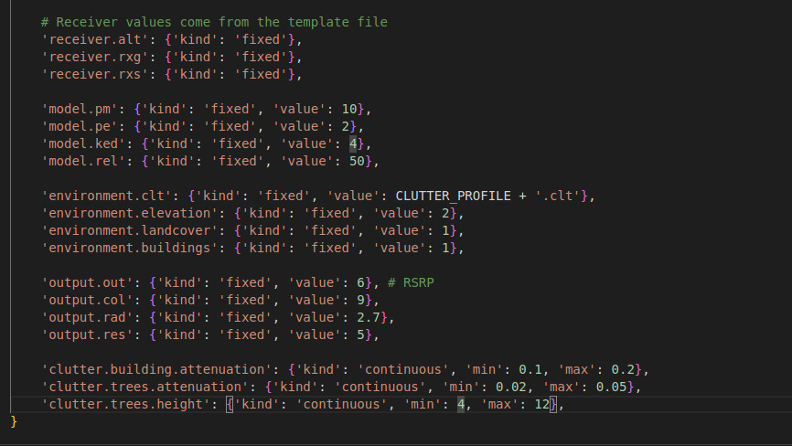
The responses are fetched as greyscale open standard GeoTIFF images which are analysed using the rasterio library against the survey measurements. The delta between points is recorded as both mean and root mean square error.

The RMSE error is the key figure which describes the error between two arrays of results. Achieving a low mean is easier to do by over-fitting a model, but lowering the RMSE is harder for a diverse environment as clutter must be tuned to allow for trees, buildings and open ground. The script constantly updates a custom clutter profile at the API with new values in between requests.

Many tools won’t publish performance data as it would make it hard to justify their price tag. Some cannot do diffraction which disqualifies them for signals below 2GHz.

The requests are scored individually using RMSE and ranked. The best scores from the generation are selected to breed the next generation and so on until the (user defined) limit is reached. Therefore, the process can be scaled to offer a quick result for a live map or a thorough result for enumeration of unknowns such as tower height, power or even tower location using a search box.

At the end of the process, the best values for the variables are shown which can either be used to build a custom clutter profile, as we do in the demo video, or scripted further to make a final layer for a third party interface.

Demo video

Conclusion

Developments in data and performance, accelerated by GPUs, means accurate and fast simulation is more viable than ever. By being able to deliver this capability in seconds instead of hours, new integrations and capabilities are possible. Furthermore using a mature API, with public examples, makes an MVP viable in days.

Using a SOOTHSAYER server, this can be done at the edge without internet access.

A few ideas for new integrations which can leverage this concept:

• A spectrum analyser with a living coverage map
• A signal classifier which shows more than metadata
• An app which shows the impact of antenna adjustments in real time
• A robot which maintains a live coverage map which can inform route selection
• An RFPS analyst can be freed up from walking around to do some analysis

Credits

Thank you to Rantcell for providing rich LTE drive test data and our resident Machine Learning guru, AppyBara, for developing our automatic calibration client. If you would like a copy get in touch.