Background

Radio Direction Finding (DF) is the art of determining the location of an emitter and is used in search and rescue, coastal surveillance, law enforcement and defence. There are different techniques using power and phase but the output for a single sensor is normally a Line of Bearing (LoB) which points towards the emitter.

If you’ve ever seen DF depicted in marketing or an info-graphic, you’ve likely seen three geometrically distributed sensors surrounding an emitter which produce a high accuracy position fix (PF) where their lines of bearing converge.

In the real world, DF systems are expensive and require specialist training so are in short supply. It is far more common for these systems to be used in isolation so operators must determine an emitter’s location with a single LoB and a map study. For powerful signals, the search area could be vast.

Guessing the signal power

For a signal to be tasked for DF, it’s frequency is already known. With signal classifiers increasingly integrated into receivers, and now even open source, the signal type may well be known which helps answer a key question: what is the signal’s transmit power?

When a new signal is detected, it could be in the room next door or in the next county. Knowing the signal type and ideally the hardware is key to estimating the distance, as you can lookup the possible power levels from a data sheet.

A portable radio has variable power levels: For a DMR radio with low and high power at 0.1W and 4W these can be put into a basic path loss model to determine the possible distance. Using the Friis reference model with a detected signal of -80dBm for example, a 1GHz signal could be 2.4km or 15km away in free space.

This significant variation with the possible distance is where modelling can add value to reduce the vast search area.

For the example radio, these power values in Watts must be converted to decibel milliwatts (dBm) for consistency with the path loss modelling and to establish the range in decibels which will inform simulation parameters. In this case, low power is 20dBm (0.1W) and high power is 36dBm (4W) for 16dB of uncertainty.

In an obstructed environment such as a forest, this uncertainty represents a shorter distance than in free space where again, modelling can add value. A counter drone system is an example of a free space problem.

Link reciprocity

A radio link is not symmetrical due to how and where obstacles impact the fresnel zone which is the cone of power an element radiates. Even if you have line of sight (LOS) between two even power stations, you can still get different received power levels from A to B than B to A.

This matters as we cannot model the emitter since we don’t know where it is! We can only model the receiver location.

In our experience, the difference is measured in single digits and is small compared with noise which will make a bigger impact on a link’s viability. If you are operating at the edge of a system’s link budget then the reciprocal difference may be enough to make a link one way only.

For modelling a receiver we need uplink (talk-in) measurements instead of downlink (talk-out) which we normally collect for clutter and model calibration.

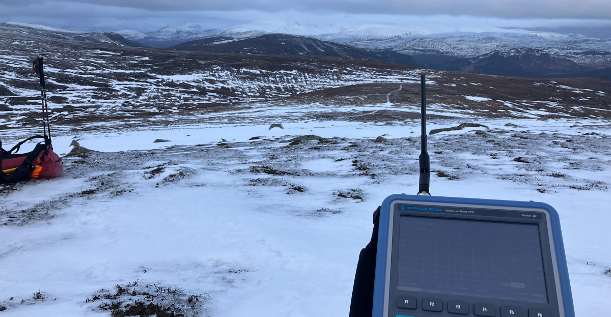
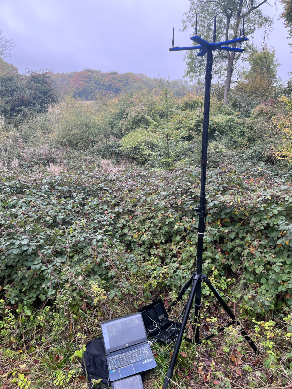
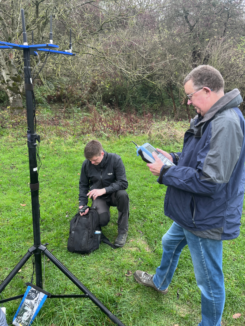
Field testing

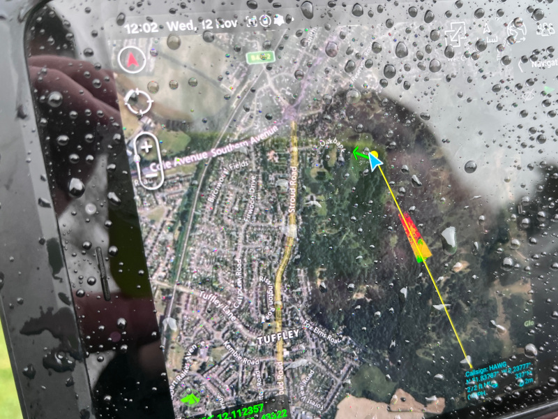
We conducted several field tests to integrate our API using a budget commercial DF receiver, the KrakenSDR. This compact entry level unit gave us a LoB (with 8 degrees of error) we could work with but as it used 8-bit SDRs, we could not rely upon the received power level as low resolution SDRs can not represent weak signals.

After a false start with a 12-bit SDR designed for the amateur community and interfaced with SoapySDR, we used a professional RFEye receiver which aside from having superior measurement accuracy and sensitivity is a turnkey solution with a web API which we have integrated with our API previously.

Test system

Our test system grew in scope from a Kraken with a Pi to a network in a box with a bespoke management and signal logging interface. Key to this innovation was not creating a budget DF system which we needed to collect data but the employment of an edge modelling capability on a Raspberry Pi 5.

Our goal was to develop a hardware agnostic script which our customers could use to enhance their DF data.

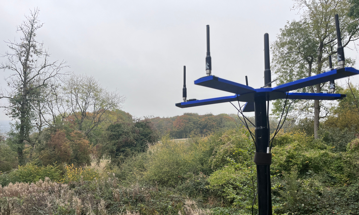
Hardware

• The Line of Bearing came from a KrakenSDR with a circular 5 element array upon a 2m telescopic mast.
• The processor was a Raspberry Pi5 running our test software and SOOTHSAYER v1.10
• The radio traffic was generated by a Tait DMR portable radio equipped with a programming cable connected to a Pi4.
• The power measurements came from a CRFS RFEye connected to an elevated monopole antenna.
• A pair of sensecap meshtastic LoRa trackers were used for GPS tracking.
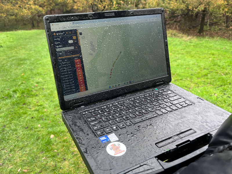
• A laptop and tablet running ATAK were used to manage the system and observe the output as a KML.

Software

To automate data collection, we developed test software to collect data from the SDR and DF receiver simultaneously and model them using our API. The DMR radio was configured to broadcast telemetry periodically which provided a regular target signal and the out-of-band meshtastic tracker provided a precise location within the trees.

We couldn’t use a second DMR radio to receive the telemetry as bi-directional radio traffic risked spoiling the data.

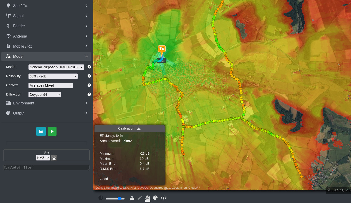
The modelling came from SOOTHSAYER 1.10 which was installed upon the Raspberry Pi 5. This also provided the map tiles for a web based logging system which displayed live signal readings. Only one (CPU) API call was necessary per test cycle to generate a grey scale Path Loss map in decibels (dB) from which subsequent received power heat maps in decibel milliwatts (dBm) could be rapidly derived using a simple formula.

The path loss simulation needs refreshing if either the location, frequency or height change but is power agnostic. The client script queries this path loss map using known (or assumed) radio power levels.

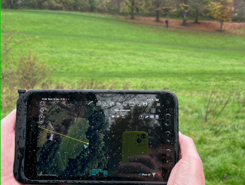
Results are presented as a network KML which can be consumed on standards based geo-viewers like ATAK.

Challenges

We took our ‘Temu DF system’ out twice but we couldn’t collect as much data as we wanted in the time available due to different constraints such as the weather or just running a small business.

A decision to avoid vehicles and buildings was made to avoid reflections which meant we had to run the equipment from travel batteries. The power budget for the Pi5 (30W), KrakenSDR (12W) and RFEye (5W) was 47W which was more than we normally test with so it reduced our endurance.

We encountered local radio traffic on our licensed channels due to the choice of locations overlooking the city. This was easy to discount at the start of the test when our signal was obvious but became a nuisance as it faded into the trees and ultimately tainted our test data since we were triggering on power.

Old data to the rescue

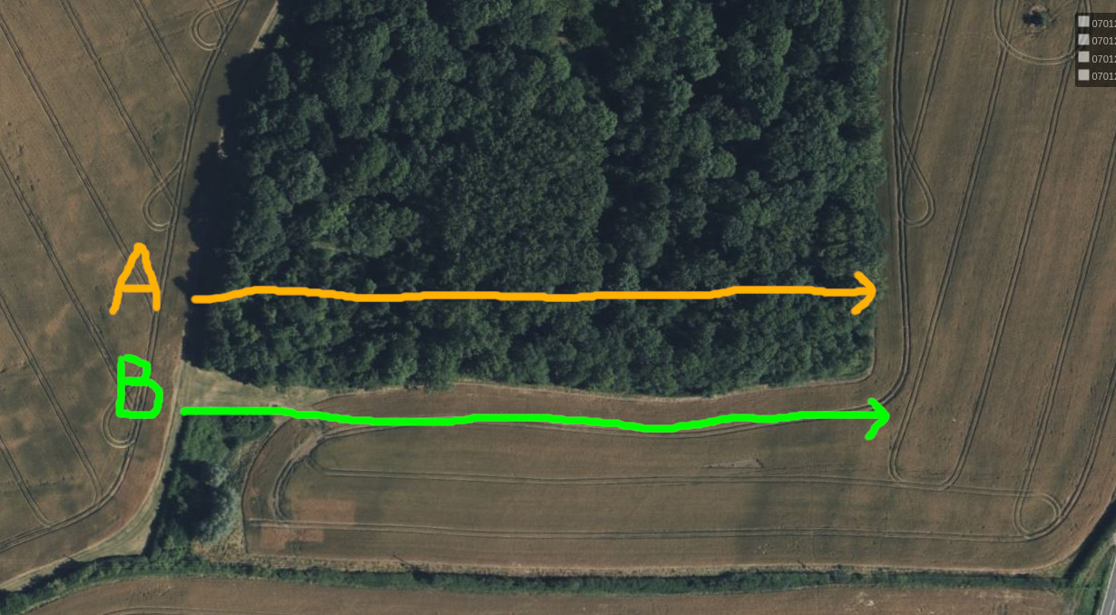
After several frustrating tests where a lot of time was spent climbing local hills, calibrating DF and chasing false positives, we elected to reuse a rich data set from an antenna field test last year which included bi-directional links for a UHF radio on a moving vehicle.

This data was attractive as it included the uplink and a good variety of obstacles including houses, trees and hills as well as LOS links which are all useful for calibration. Before we could conduct DF analysis with the uplink, we calibrated the local clutter using the downlink, as we do routinely for calibration. This is a standard process we have developed a feature for in the web interface as well as a supporting video tutorial. Using our new 2m tree height data, we were able to improve upon last year’s score.

As we did not collect lines of bearings during that model test, we had to simulate these using the known vehicle location for which we used 10 degrees of azimuth error.

Analysis technique

To compute the effectiveness of this technique we calculated the area of the 10 degree arc where the vehicle could have been, with a radius of 6km representing the maximum range in this test.

This gave us a search area for a given LoB of 3,141,593 m2.

Our analysis script calculated a high resolution grey scale heatmap using SOOTHSAYER’s API which was referenced with collected power readings. To compare path loss (dB) with received power (dBm) we used the known radio power of 2W (33dBm) within a link budget formula to generate received power which was compared with measurements.

RSSI (dBm) = Radio Power (dBm) + Gain (dBi) - Path Loss (dB) - Losses (dB) + Receiver Gain (dBi) - Receiver Loss (dB)

Where the difference between measurements and simulation was within tolerances of our colour key, we styled that pixel, otherwise we eliminate it from the search area and set it to transparent.

The result is an accuracy heatmap defined by a traffic light colour key. The levels we chose for our “known power” assessment were 1, 2 and 3dB. By showing 3dB of error we allow for receiver error and reduce the risk of false negatives where a matching location might be discounted.

When the radio power is known, we can produce more accurate results.

When the radio power is unknown and the hardware/signal is known, we can simulate the minimum and maximum power to generate a dynamic range for the analysis. We used a low power value of 20dBm (0.1W) and a high power value of 36dBm (4W) for a possible power range of 16dB so our “low accuracy” colour key was 14/15/16dB.

We repeated the analysis with known and unknown power levels to compare accuracy.

Results

Analysis of data revealed the simulation heatmap significantly reduced the search area. As expected, knowing the radio power helps greatly but even with unknown power the search area was reduced to 32% of what it could have been for a conventional 6km arc.

Even when radio power is unknown, the search area is reduced significantly

	Known Power (2W)	Unknown Power (0.1 or 4W)
Best case	0.01	0.03
Worst case	27.33	64.37
Average area	7.93%	31.51%

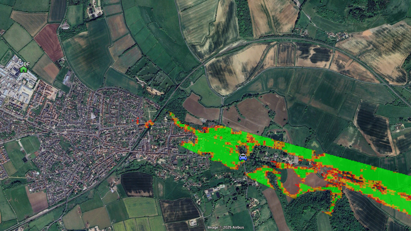
The amount of benefit was relative to the terrain and clutter: For example, where there were no obstacles or a single consistent obstacle such as a forest, the result was a focused band of probability without any false positives.

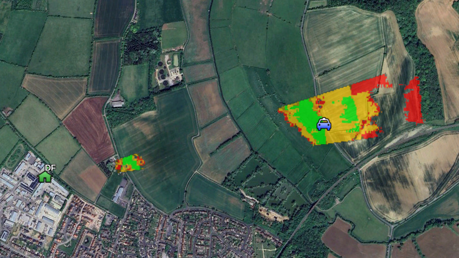
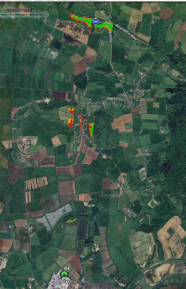
Where there were multiple obstacles such as a hill and a forest, false positives appeared which depending upon the ground could be discounted by an observer. This was to be expected given the pixel picking which is taking place.

A tight traffic light schema, with tuned clutter, was better than a loose schema with larger error margins. The reason being that it will show much less false positives.

Video and KMZ

This video is a sped-up compilation of time stamped KMZ layers viewed on Google Earth showing the vehicle’s route around the sensor. Where the vehicle disappears, no signal was detected.

The KMZ is available here and works best in Google Earth.

Conclusion

This testing proved that the effectiveness of a single LoB can be improved greatly with modelling but the concept is only an improvement if the analysis is automated as doing this manually would not be faster than a map study.

The reason this analysis isn’t performed regularly by DF systems today isn’t for a lack of LoBs and RSSI measurements but rather a lack of APIs with which to exploit this information. Current RF planning software exists as a user interface which requires manual, and skilled, operation. Furthermore, the capability often exists in the wrong location on a high performance desktop computer, disconnected from edge sensors.

By putting this API at the edge on small board computers (SBCs) such as the Raspberry Pi 5 or Nvidia Jetson, a DF system’s effectiveness can be improved. Through open GIS standards like KML, the result can be consumed on open standard GIS systems like ATAK requiring minimal integration effort to add a powerful capability.

Looking forward, we are speaking with open minded vendors about adding this API to enhance existing systems.

If you’d like to improve your LoBs, get in touch with us or one of our regional resellers.

Links

SOOTHSAYER server: https://cloudrf.com/soothsayer

Kraken SDR: https://www.krakenrf.com/

DF integration demo: https://github.com/Cloud-RF/CloudRF-API-clients/tree/master/integrations/DF

API schema: https://cloudrf.com/documentation/developer