How Can We Help?
3D interface user guide
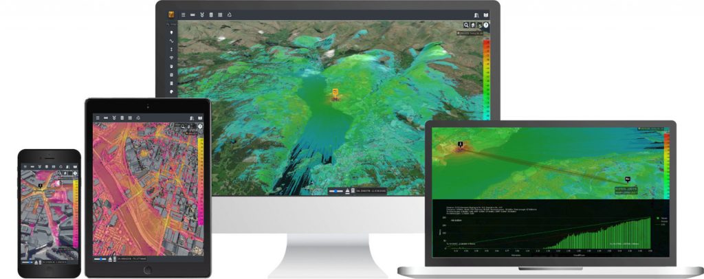
The 3D interface is the primary user interface for CloudRF and works on desktops, tablets and mobiles.
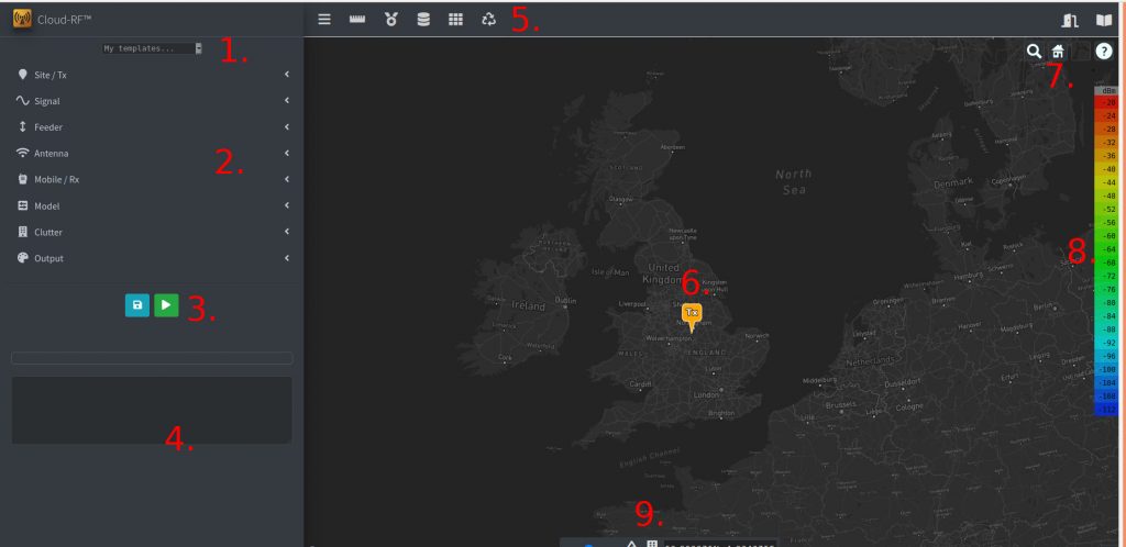
| Number | Description |
|---|---|
| 1 | Templates |
| 2 | Input menu |
| 3 | Save / Run buttons |
| 4 | Output console |
| 5 | Function menu |
| 6 | Transmitter location marker |
| 7 | Address lookup, Mapping select |
| 8 | Colour key |
| 9 | Opacity slider, 3D terrain, 3D buildings toggles |
Template
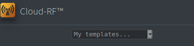
Templates allows you to quickly apply settings from a saved configuration. Anytime you use the ‘Save’ button at the bottom of the menu it will create a template which you can give a user friendly name eg. “Radio X”. This is useful in a shared account where an Engineer might prepare the template(s) and a sales person might use them to qualify customers.
Input menu
The accordion style input menu has collapsible sections to allow you to focus on settings, grouped into the following categories.
Site Menu
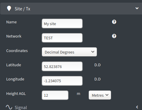
The site menu contains settings relating to the physical location of the antenna relative to the ground and the Name and parent Network of the site. These settings will be of increasing importance as your network grows and you need to perform analysis such as “best server”.
Location can be entered manually or set by clicking upon the map. Decimal degrees, Degrees/Minutes/Seconds and NATO MGRS inputs are all acceptable and the system will convert between them.
Distance units are set here which apply to all heights and radius. The system default is metres and kilometres. Choosing Feet will set distance calculations to Miles.
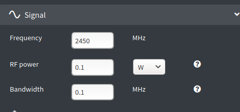
The signal menu contains settings relating the actual radiation such as frequency in Megahertz, transmitter power (Not ERP/EIRP yet) and the bandwidth.
Bandwidth will affect channel noise and Signal-to-Noise ratio. The system will compensate for wide-band noise by making adjustments to receiver sensitivity in line with Shannon’s theorem so a wideband signal won’t appear to go as far as a narrow one – but the ERP / EIRP is untouched.
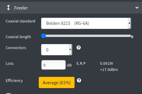
The feeder menu relates to cabling and connectors between a transmitter and a radio. It’s an easy mistake to think mounting an antenna higher makes for a better signal but this theory only stands if you’re working lower frequencies or have some very thick ‘low loss’ cable.
For UHF signals above 300MHz, feeder loss is a significant issue which must be budgeted carefully. Even a few metres of coaxial could reduce your system efficiency by 50%.
This is also where Effective Radiated Power (ERP) is dynamically calculated. This figure will change as you manipulate powers and gains on the interface, along with an efficiency label to show how your system performs as a ratio of input to actual output.
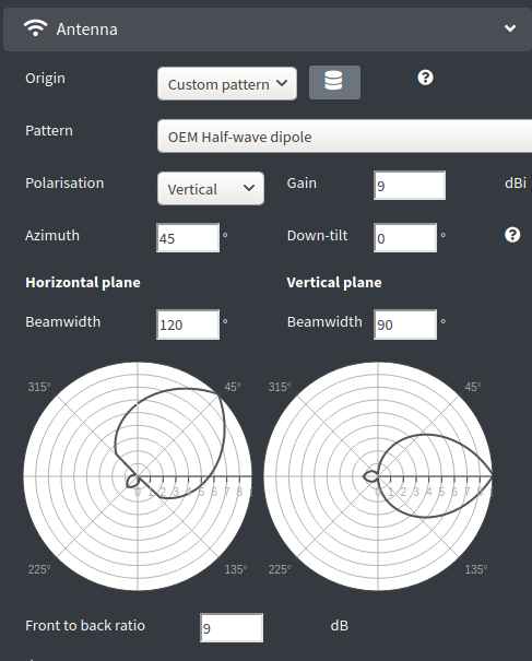
The antennas menu lets you choose or build an antenna.
You have a choice at the top of a template from your chosen list or a custom pattern. To define your templates list open the antenna archive via the adjacent button. Within here you can find or upload patterns as ADF files. Select the patterns you like to add them to your list and refresh the interface to have them populate in your list.
A custom pattern lets you build an antenna using beamwidth values in degrees. You can set the horizontal and vertical beamwidth, gain, front-to-back ratio (use gain if unsure), down-tilt relative to the horizon and finally azimuth relative to true north.
The polar plots will update as you change the settings so you can see if it looks right.
The peak gain is measured in decibel-isotropic (dBi) and will affect ERP (see feeder menu).
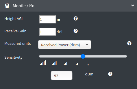
The Mobile / Receiver menu contains settings relating to the other end of the link. This could be a mobile outstation, a customer or a vehicle.
Height in metres or feet is height of the antenna above the ground. Use 1 or 2m for a handheld radio. Height units are defined in the site menu.
The receive gain (dBi) is the combined receiver and antenna gain. If the receiver has a 3dBi antenna and a 3dBi receiver noise figure this would be 0dBi. Use 1dBi for a mobile phone. Actual performance varies by band so a phone may have 2dBi gain for GSM900 but 1dBi for UMTS-2100.
The measured units are in either dB, dBm or dBuV/m and must correspond with the chosen colour key if performing area coverage plots.
The sensitivity slider lets you define the sensitivity of the mobile station in units corresponding to the measured units. For a mobile phone with received power this would have a limit of around -105dBm. Setting this too low eg. -120dBm would result in an unrealistic prediction unless your system is designed to function that low. IoT protocols like LoRa LPWAN can theoretically operate down to -140dBm but this is under ideal conditions. In the real, noisy world most digital communications bottom out at between -100 and -115dBm. Adding a 10dB error margin gives a recommended range of -90 to -105dBm for sensitivity.
Save, Run buttons
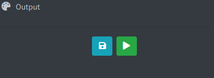
Beneath the input menu are two buttons, save and run.
Save will let you create a template for reuse later on using all the settings you have entered.
Run will execute a coverage calculation using your settings which typically results in a progress bar and a delay of several seconds, depending on resolution and radius.
Output console
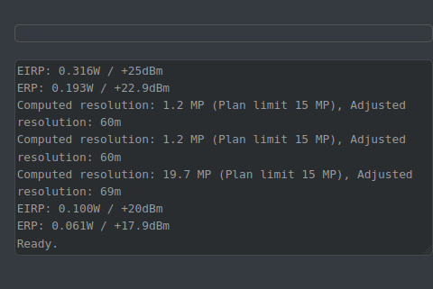
The output console provides useful feedback as you use the tool relating to settings, errors, API inputs and API outputs.
Effective radiated power and computed resolution in mega-pixels will be printed in this console as you adjust settings so you should keep an eye on it.
When you submit a calculation for processing all the API parameters are visible so if you are a developer you can copy paste them for use in your code.
As an area calculation processes you will see periodic updates in the console from the SLEIPNIR propagation engine.
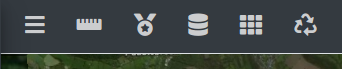
Function menu
The function menu lives at the top of the interface and has several key functions.
The menu bars let you hide the side menu, the ruler opens the path profile (PtP) tool, the medal is the best server tool; useful checking for coverage against an established network, the database icon opens your archive, the grid icon is the mesh tool which lets you generate a new superlayer composed of different layers from the same network eg. “MY NETWORK”.
Finally the recycle icon will clear and reset the map of all layers. Layers can be reloaded from within your archive.
Transmitter marker
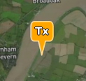
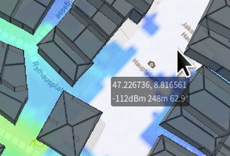
The transmitter marker (Tx) designates your antenna location. Clicking on the map will move this marker and update your location settings within the input menu. When you have a layer the information box next to to the cursor will display the current co-ordinates, signal strength, distance and angle from the site.
Mapping selection
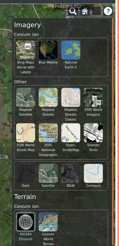
In the top right corner you can search for addresses or change the mapping / imagery.
Choices offered include satellite imagery, street mapping and high contrast ‘dark’ layers for use with colourful overlays.
You can also enable and disable the underlying 3D terrain here. By default 3D terrain is hidden to improve performance but this can be enabled by clicking the mountain icon at the bottom centre of the screen.
Colour key
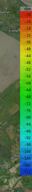
The colour key on the right denotes signal levels. It can be changed by switching the colour key in the Output menu.
This key only applies to area coverage plots and can be in dB, dBm or dBuV/m.
To change the actual colours and values in the key, open the ‘My colours’ tool from within the Output menu. Here you can build and edit colour keys, set levels, change colours and define limits.
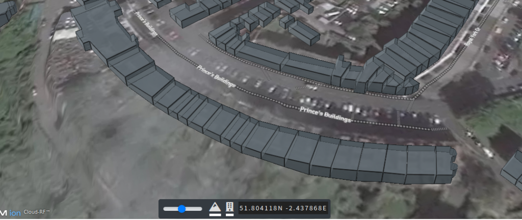
Map tools, 3D terrain & buildings
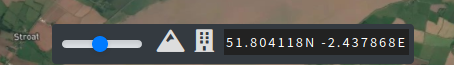
The map tools at the bottom let you set the layer(s) opacity with a slider, enable/disable 3D terrain and enable/disable 3D buildings. For performance 3D layers are disabled by default but only in the 3D viewer, this does not apply to the API.
The location box will display the Tx cursors location in decimal degrees. This is a duplication of information in the menu in case you have it closed.
Clicking 3D buildings will enable 3D terrain also. When enabled the buttons will be highlighted with a white bar.