


Reference Data
Antenna Patterns
The antenna database lets you search for patterns by manufacturer, model and/or physical parameters like gain.
To access the Antenna Database:
Under the Antenna Input menu, click on the Manage my Antennas
 icon.
icon.The Antenna Database dialog box will appear. You can choose to open this in a separate tab with the hyperlink at the bottom.
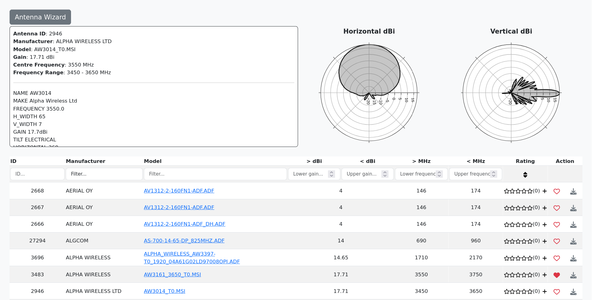
In the table, you can search the Antenna Database by filtering on parameters.
To do so:
Select the desired Manufacturer.
The respective manufacturer’s list of Antenna Patterns will be displayed.
Select the desired Model.
The respective Antenna Pattern’s information - ID, Name, Description, Frequency, Gain, Polarisation and Polar Maps will be displayed once a row is clicked.
Choosing a favourite pattern
Each row has a heart icon to the right. Click the heart to ‘favourite’ a pattern and click it again to ‘unfavourite’ it.


When a pattern is a favourite, the heart will be red and it will appear on your list within 10 seconds.
Antenna pattern data
At the top of the atenna database interface there is a link to the Antenna Wizard.
The wizard can be used to:
Upload antenna patterns for use in calculations,
Convert antenna patterns to TIA/EIA-804-B (NSMA) ADF format.
The wizard works with ADF, MSI and ANT formats. The patterns can be flipped, swapped, and rotated.
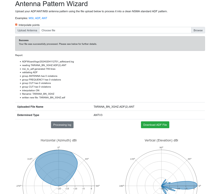
Some ADF files contain multiple patterns for the same antenna, different patterns for different frequencies and polarizations. Currently, the system treats these as seperate patterns so the must be uploaded separately.
For more information see Antenna patterns.
To validate an ADF pattern use our online tool here: https://api.cloudrf.com/API/antennas/validator/index.php
Example TIA/EIA-804-B pattern file
This example data shows the unique colon-comma formatting this TIA standard uses. It might not make sense compared with modern information standards but it is a ratified standard and is widely supported as a result.
REVNUM:,TIA/EIA-804-B
COMNT1:,Standard TIA/EIA Antenna Pattern Data
ANTMAN:,RFI Antennas for Bird Technologies Group
MODNUM:,CC806-06 @ 870
DESCR1:,Corporate collinear, 746-870 MHz
DESCR2:,Omnidirectional, 5dBd, 0o Downtilt
DTDATA:,20060213
LOWFRQ:,746
HGHFRQ:,870
GUNITS:,DBD/DBR
MDGAIN:,4.8
AZWIDT:,360
ELWIDT:,17
CONTYP:,7/16 DIN Silver Plated
ATVSWR:,1.5
FRTOBA:,0
ELTILT:,0
MAXPOW:,500
ANTLEN:,1.85
ANTWID:,0.077
ANTWGT:,7.1
PATTYP:,Typical
NOFREQ:,1
PATFRE:,870
NUMCUT:,2
PATCUT:,V
POLARI:,V/V
NUPOIN:,360
FSTLST:,-179,180
-179,-0.053
-178,-0.179
-177,-0.374
-176,-0.639
-175,-0.971
-174,-1.376
-173,-1.857
-172,-2.425
-171,-3.089
-170,-3.866
-169,-4.772
-168,-5.831
-167,-7.069
-166,-8.515
-165,-10.202
-164,-12.146
-163,-14.296
-162,-16.376
-161,-17.699
-160,-17.679
-159,-16.748
-158,-15.657
-157,-14.757
-156,-14.132
-155,-13.777
-154,-13.665
-153,-13.770
-152,-14.066
-151,-14.532
-150,-15.146
-149,-15.888
-148,-16.736
-147,-17.668
-146,-18.656
-145,-19.667
-144,-20.654
-143,-21.546
-142,-22.234
-141,-22.588
-140,-22.512
-139,-22.014
-138,-21.214
-137,-20.261
-136,-19.278
-135,-18.338
-134,-17.483
-133,-16.730
-132,-16.084
-131,-15.544
-130,-15.107
-129,-14.767
-128,-14.520
-127,-14.358
-126,-14.277
-125,-14.271
-124,-14.337
-123,-14.468
-122,-14.662
-121,-14.914
-120,-15.221
-119,-15.579
-118,-15.986
-117,-16.439
-116,-16.935
-115,-17.472
-114,-18.048
-113,-18.659
-112,-19.305
-111,-19.982
-110,-20.689
-109,-21.424
-108,-22.185
-107,-22.972
-106,-23.782
-105,-24.618
-104,-25.481
-103,-26.374
-102,-27.304
-101,-28.282
-100,-29.320
-99,-30.441
-98,-31.672
-97,-33.053
-96,-34.640
-95,-36.507
-94,-38.739
-93,-41.001
-92,-41.317
-91,-43.387
-90,-43.536
-89,-43.387
-88,-41.317
-87,-41.001
-86,-38.739
-85,-36.507
-84,-34.640
-83,-33.053
-82,-31.672
-81,-30.441
-80,-29.320
-79,-28.282
-78,-27.304
-77,-26.374
-76,-25.481
-75,-24.618
-74,-23.782
-73,-22.972
-72,-22.185
-71,-21.424
-70,-20.689
-69,-19.982
-68,-19.305
-67,-18.659
-66,-18.048
-65,-17.472
-64,-16.935
-63,-16.439
-62,-15.986
-61,-15.579
-60,-15.221
-59,-14.914
-58,-14.662
-57,-14.468
-56,-14.337
-55,-14.271
-54,-14.277
-53,-14.358
-52,-14.520
-51,-14.767
-50,-15.107
-49,-15.544
-48,-16.084
-47,-16.730
-46,-17.483
-45,-18.338
-44,-19.278
-43,-20.261
-42,-21.214
-41,-22.014
-40,-22.512
-39,-22.588
-38,-22.234
-37,-21.546
-36,-20.654
-35,-19.667
-34,-18.656
-33,-17.668
-32,-16.736
-31,-15.888
-30,-15.146
-29,-14.532
-28,-14.066
-27,-13.770
-26,-13.665
-25,-13.777
-24,-14.132
-23,-14.757
-22,-15.657
-21,-16.748
-20,-17.679
-19,-17.699
-18,-16.376
-17,-14.296
-16,-12.146
-15,-10.202
-14,-8.515
-13,-7.069
-12,-5.831
-11,-4.772
-10,-3.866
-9,-3.089
-8,-2.425
-7,-1.857
-6,-1.376
-5,-0.971
-4,-0.639
-3,-0.374
-2,-0.179
-1,-0.053
0,0.000
1,-0.080
2,-0.200
3,-0.700
4,-1.300
5,-1.987
6,-2.509
7,-3.159
8,-3.946
9,-4.882
10,-5.982
11,-7.264
12,-8.756
13,-10.498
14,-12.551
15,-15.021
16,-18.110
17,-22.259
18,-28.598
19,-34.203
20,-27.412
21,-23.162
22,-20.560
23,-18.783
24,-17.499
25,-16.553
26,-15.866
27,-15.396
28,-15.122
29,-15.033
30,-15.127
31,-15.406
32,-15.876
33,-16.547
34,-17.431
35,-18.537
36,-19.862
37,-21.359
38,-22.862
39,-23.992
40,-24.280
41,-23.680
42,-22.631
43,-21.539
44,-20.590
45,-19.839
46,-19.287
47,-18.922
48,-18.725
49,-18.682
50,-18.776
51,-18.997
52,-19.333
53,-19.771
54,-20.300
55,-20.905
56,-21.568
57,-22.264
58,-22.963
59,-23.627
60,-24.216
61,-24.695
62,-25.041
63,-25.251
64,-25.343
65,-25.345
66,-25.294
67,-25.220
68,-25.146
69,-25.091
70,-25.066
71,-25.076
72,-25.125
73,-25.214
74,-25.343
75,-25.509
76,-25.711
77,-25.945
78,-26.210
79,-26.502
80,-26.818
81,-27.154
82,-27.506
83,-27.871
84,-28.243
85,-28.617
86,-29.000
87,-30.000
88,-31.000
89,-34.000
90,-36.000
91,-34.000
92,-31.000
93,-30.000
94,-29.000
95,-28.617
96,-28.243
97,-27.871
98,-27.506
99,-27.154
100,-26.818
101,-26.502
102,-26.210
103,-25.945
104,-25.711
105,-25.509
106,-25.343
107,-25.214
108,-25.125
109,-25.076
110,-25.066
111,-25.091
112,-25.146
113,-25.220
114,-25.294
115,-25.345
116,-25.343
117,-25.251
118,-25.041
119,-24.695
120,-24.216
121,-23.627
122,-22.963
123,-22.264
124,-21.568
125,-20.905
126,-20.300
127,-19.771
128,-19.333
129,-18.997
130,-18.776
131,-18.682
132,-18.725
133,-18.922
134,-19.287
135,-19.839
136,-20.590
137,-21.539
138,-22.631
139,-23.680
140,-24.280
141,-23.992
142,-22.862
143,-21.359
144,-19.862
145,-18.537
146,-17.431
147,-16.547
148,-15.876
149,-15.406
150,-15.127
151,-15.033
152,-15.122
153,-15.396
154,-15.866
155,-16.553
156,-17.499
157,-18.783
158,-20.560
159,-23.162
160,-27.412
161,-34.203
162,-28.598
163,-22.259
164,-18.110
165,-15.021
166,-12.551
167,-10.498
168,-8.756
169,-7.264
170,-5.982
171,-4.882
172,-3.946
173,-3.159
174,-2.509
175,-1.987
176,-1.300
177,-0.700
178,-0.200
179,-0.080
180,0.000
PATCUT:,H
POLARI:,V/V
NUPOIN:,360
FSTLST:,-179,180
-179,-1.097
-178,-1.096
-177,-1.095
-176,-1.094
-175,-1.091
-174,-1.088
-173,-1.085
-172,-1.080
-171,-1.075
-170,-1.070
-169,-1.064
-168,-1.057
-167,-1.050
-166,-1.043
-165,-1.034
-164,-1.026
-163,-1.017
-162,-1.007
-161,-0.998
-160,-0.987
-159,-0.977
-158,-0.966
-157,-0.955
-156,-0.944
-155,-0.933
-154,-0.921
-153,-0.910
-152,-0.898
-151,-0.887
-150,-0.875
-149,-0.863
-148,-0.852
-147,-0.841
-146,-0.829
-145,-0.818
-144,-0.807
-143,-0.797
-142,-0.786
-141,-0.776
-140,-0.766
-139,-0.756
-138,-0.747
-137,-0.738
-136,-0.730
-135,-0.721
-134,-0.713
-133,-0.706
-132,-0.699
-131,-0.692
-130,-0.685
-129,-0.679
-128,-0.673
-127,-0.668
-126,-0.662
-125,-0.658
-124,-0.653
-123,-0.649
-122,-0.644
-121,-0.640
-120,-0.637
-119,-0.633
-118,-0.630
-117,-0.627
-116,-0.623
-115,-0.620
-114,-0.617
-113,-0.614
-112,-0.611
-111,-0.608
-110,-0.605
-109,-0.602
-108,-0.599
-107,-0.595
-106,-0.592
-105,-0.588
-104,-0.584
-103,-0.580
-102,-0.576
-101,-0.571
-100,-0.566
-99,-0.561
-98,-0.556
-97,-0.550
-96,-0.544
-95,-0.538
-94,-0.531
-93,-0.524
-92,-0.516
-91,-0.509
-90,-0.501
-89,-0.492
-88,-0.484
-87,-0.474
-86,-0.465
-85,-0.455
-84,-0.445
-83,-0.435
-82,-0.424
-81,-0.413
-80,-0.402
-79,-0.391
-78,-0.379
-77,-0.367
-76,-0.355
-75,-0.343
-74,-0.330
-73,-0.318
-72,-0.305
-71,-0.293
-70,-0.280
-69,-0.268
-68,-0.255
-67,-0.242
-66,-0.230
-65,-0.217
-64,-0.205
-63,-0.193
-62,-0.181
-61,-0.170
-60,-0.158
-59,-0.147
-58,-0.136
-57,-0.125
-56,-0.115
-55,-0.105
-54,-0.096
-53,-0.087
-52,-0.078
-51,-0.070
-50,-0.062
-49,-0.055
-48,-0.048
-47,-0.041
-46,-0.035
-45,-0.030
-44,-0.025
-43,-0.020
-42,-0.016
-41,-0.013
-40,-0.010
-39,-0.007
-38,-0.005
-37,-0.003
-36,-0.002
-35,-0.001
-34,0.000
-33,0.000
-32,0.000
-31,-0.001
-30,-0.002
-29,-0.003
-28,-0.004
-27,-0.006
-26,-0.008
-25,-0.010
-24,-0.012
-23,-0.014
-22,-0.017
-21,-0.020
-20,-0.022
-19,-0.025
-18,-0.028
-17,-0.031
-16,-0.034
-15,-0.037
-14,-0.039
-13,-0.042
-12,-0.045
-11,-0.047
-10,-0.049
-9,-0.052
-8,-0.054
-7,-0.056
-6,-0.057
-5,-0.059
-4,-0.060
-3,-0.061
-2,-0.062
-1,-0.062
0,-0.063
1,-0.063
2,-0.063
3,-0.062
4,-0.062
5,-0.061
6,-0.060
7,-0.059
8,-0.057
9,-0.056
10,-0.054
11,-0.052
12,-0.049
13,-0.047
14,-0.045
15,-0.042
16,-0.039
17,-0.037
18,-0.034
19,-0.031
20,-0.028
21,-0.025
22,-0.022
23,-0.020
24,-0.017
25,-0.014
26,-0.012
27,-0.010
28,-0.008
29,-0.006
30,-0.004
31,-0.003
32,-0.002
33,-0.001
34,0.000
35,0.000
36,0.000
37,-0.001
38,-0.002
39,-0.003
40,-0.005
41,-0.007
42,-0.010
43,-0.013
44,-0.016
45,-0.020
46,-0.025
47,-0.030
48,-0.035
49,-0.041
50,-0.048
51,-0.055
52,-0.062
53,-0.070
54,-0.078
55,-0.087
56,-0.096
57,-0.105
58,-0.115
59,-0.125
60,-0.136
61,-0.147
62,-0.158
63,-0.170
64,-0.181
65,-0.193
66,-0.205
67,-0.217
68,-0.230
69,-0.242
70,-0.255
71,-0.268
72,-0.280
73,-0.293
74,-0.305
75,-0.318
76,-0.330
77,-0.343
78,-0.355
79,-0.367
80,-0.379
81,-0.391
82,-0.402
83,-0.413
84,-0.424
85,-0.435
86,-0.445
87,-0.455
88,-0.465
89,-0.474
90,-0.484
91,-0.492
92,-0.501
93,-0.509
94,-0.516
95,-0.524
96,-0.531
97,-0.538
98,-0.544
99,-0.550
100,-0.556
101,-0.561
102,-0.566
103,-0.571
104,-0.576
105,-0.580
106,-0.584
107,-0.588
108,-0.592
109,-0.595
110,-0.599
111,-0.602
112,-0.605
113,-0.608
114,-0.611
115,-0.614
116,-0.617
117,-0.620
118,-0.623
119,-0.627
120,-0.630
121,-0.633
122,-0.637
123,-0.640
124,-0.644
125,-0.649
126,-0.653
127,-0.658
128,-0.662
129,-0.668
130,-0.673
131,-0.679
132,-0.685
133,-0.692
134,-0.699
135,-0.706
136,-0.713
137,-0.721
138,-0.730
139,-0.738
140,-0.747
141,-0.756
142,-0.766
143,-0.776
144,-0.786
145,-0.797
146,-0.807
147,-0.818
148,-0.829
149,-0.841
150,-0.852
151,-0.863
152,-0.875
153,-0.887
154,-0.898
155,-0.910
156,-0.921
157,-0.933
158,-0.944
159,-0.955
160,-0.966
161,-0.977
162,-0.987
163,-0.998
164,-1.007
165,-1.017
166,-1.026
167,-1.034
168,-1.043
169,-1.050
170,-1.057
171,-1.064
172,-1.070
173,-1.075
174,-1.080
175,-1.085
176,-1.088
177,-1.091
178,-1.094
179,-1.095
180,-1.096
ENDFIL:,EOF
Antenna pattern test range
As well as testing over water, the Meteor crater west of Winslow, Arizona is recommended for proving vertical antenna patterns as the elevation plane can be seen clearly on the walls.
Terrain data
The system works with raster data in the GeoTIFF format with WGS-84 projection.
SOOTHSAYER users with a private server can add their own tiles by placing them in the mapped /data/DEM/ folder and importing them within the admin dashboard. See the SOOTHSAYER documentation for more information on adding your own data.
GeoTIFF tiles need to be of type Int16 in WGS-84 (EPSG:4326) projection with a pixel resolution of between 1 and 30m. LZW compression is recommended.
For a map of current CloudRF system data see Terrain data map. Data is continuously added and refreshed so this is a live map.
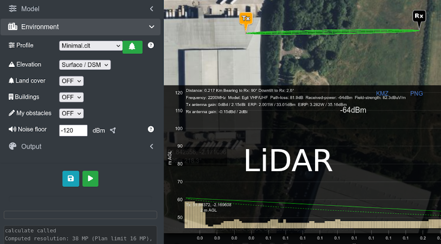
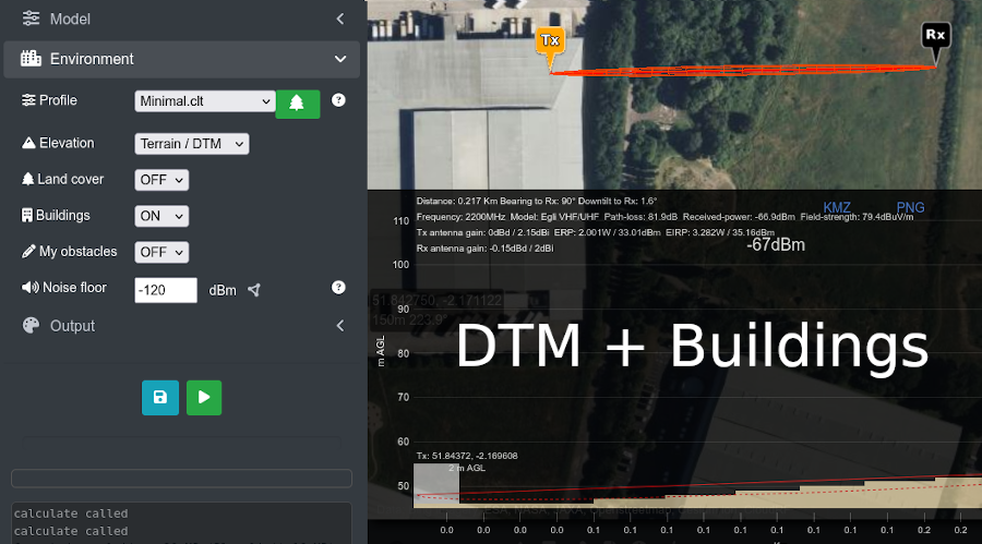
Buildings and LiDAR
When using LiDAR data, users should be aware that it is a single surface layer (DSM) which includes buildings. Therefore if you need a 2m mast on top of a 9m building this is still a relative height of 2m for the input form.
To test for LiDAR, use the path tool with DSM and without the buildings layer at high resolution eg. 5m. If you see buildings you have LiDAR in your area.
If you do not have LiDAR, use the digital terrain model (DTM), which describes most of the earth, and enter an absolute height above ground of 11m to simulate a 2m mast atop a 9m building.
In the web interface, LiDAR data is used when the terrain type is DSM and the resolution is <= 30m. If it is not available, a 30m DSM model will be used. This does not contain buildings so must be enhanced with the buildings layer.
In these images, a 2m high antenna is modelled using DSM LiDAR and DTM with buildings. Note the DTM link appears obstructed since it is inside the obstacle so needs elevating to the absolute height of 11m above ground to budget for the 9m building.
Clutter data
The system has several forms of landcover data to enhance above surface accuracy, especially in urban areas.
All users can draw and self-classify private clutter items in the web interface as polylines or polygons. Using this technique you can represent almost any obstacle from light trees through to concrete and solid metal.
Large numbers of obstacles can be uploaded as KML or GeoJSON in the web interface.
Uploaded clutter belongs to a user and is not visible to others.
For more information on landcover classes see Clutter data.
10m Landcover
The primary clutter source is European Space Agency (ESA) 10m Landcover data, published in October 2021.
WorldCover provides a new baseline global land cover product at 10 m resolution for 2020 based on Sentinel-1 and 2 data that was developed and validated in almost near-real time and at the same time maximizes the impact and uptake for the end users.
A tremendous step forward towards the joint use of Sentinel satellite data for worldwide land cover mapping.
© ESA WorldCover project 2020 / Contains modified Copernicus Sentinel data (2020) processed by ESA WorldCover consortium
This comprehensive dataset covers the planet and has 9 bands for Trees, Shrubland, Grassland, Crops, Built-up, Bare ground, Snow/Ice, Water, Swamps and Mangroves.
WARNING: Be careful when setting the ‘urban’ landcover height since this elevates roads (and car parks etc) as well as buildings! Keep this height low and use the buildings layer instead for urban planning.
3D Buildings
A supplementary clutter source are 3D Buildings, derived from satellite imagery using machine learning. These are accurate to 2m and have better global coverage than crowd sourced equivalents.
The height of buildings is either estimated or crowd sourced. Where height is unknown an approximate local value is used based upon neighbour heights. The minimum height is 3m.
Custom Clutter
All users can draw and self-classify private clutter items in the web interface as polylines or polygons. Using this technique you can represent almost any obstacle from light trees through to concrete.
Large numbers of obstacles can be uploaded as KML or GeoJSON in the web interface.
Uploaded clutter belongs to a user or the system. VM administrators can override clutter ownership manually in the SQL clutter table to make it system clutter for the benefit of all users.
For more information on land cover classes see Clutter data.
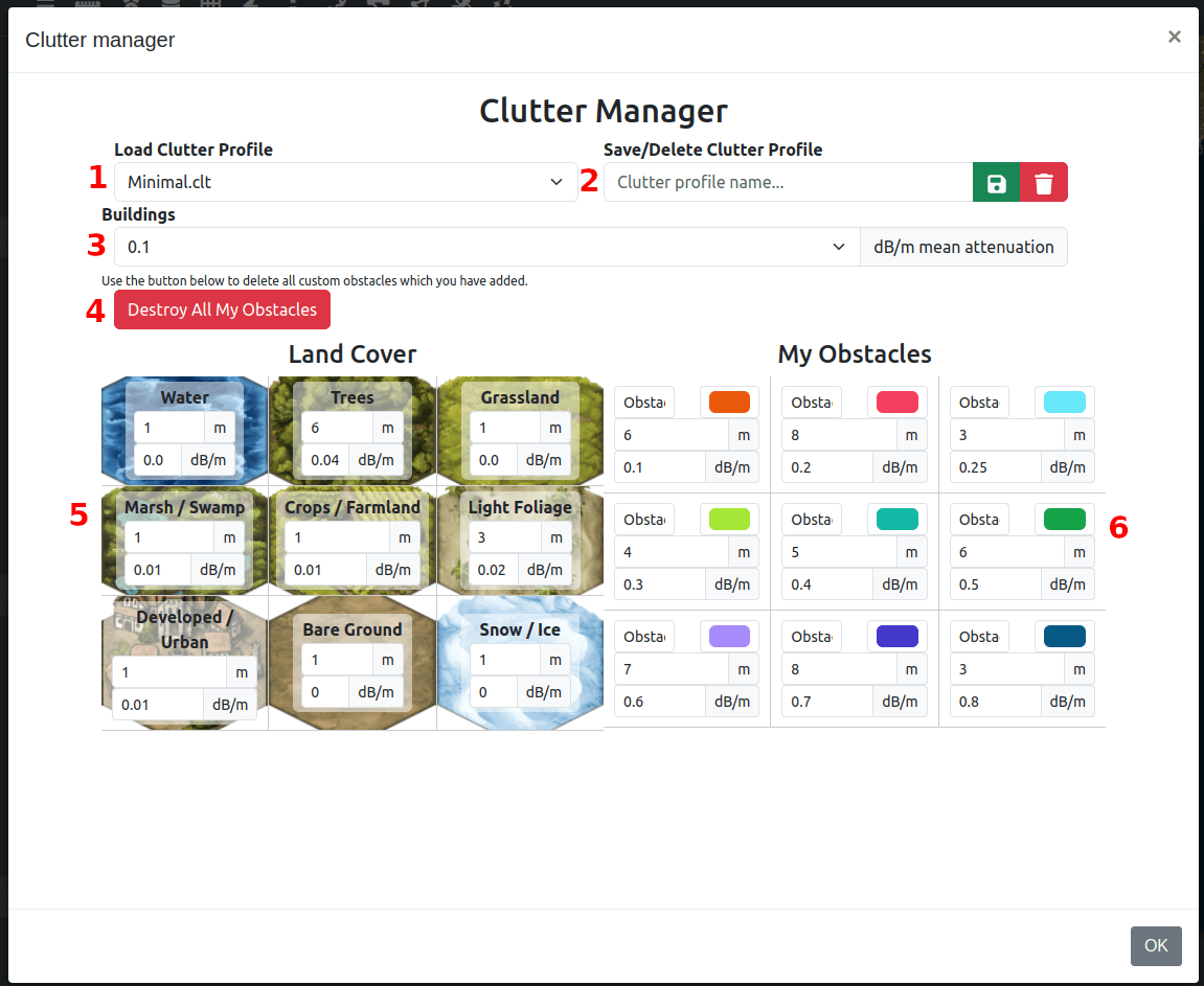
Selected clutter profile
Save/delete profile as name
Building attenuation
Delete all obstacles on your account
Land cover types with customisable height and attenuation values
My obstacle (clutter) types with customisable name, colour, height and attenuation values
Clutter codes
In a clutter profile the codes represent different types of landcover.
System Landcover
1Water2Trees3Grassland4Swamp5Crops6Shrubland7Built-up8Bare ground9Snow / Ice
Custom Clutter
Codes 11 through 19 represent “Custom Clutter”. These codes are free to be customised as per your particular usecase and environment. You have the ability to define a name and a colour for each of these clutter codes which will be represented in calculations.
For more information on how to add clutter with these codes, please consult the clutter documentation.
Clutter Profiles
Premium users can define custom clutter profiles for regions eg. AFRICA.clt, POLAND.clt. These are saved within your folder as .clt files. VM users can add these locally by placing .clt files in the folder.
A .clt is a simple text format with tab delimiters and 3 columns: “Code”, “Height (m)” and “Nominal Attenuation (dB/m)”.
Codes 11 through 19 represent your “My Obstacles” and also have 2 additional columns of “Name” and “Colour Code”. This allows you to customise your custom obstacles further.
The system default, Minimal.clt, looks like this. Code 10 is not used.
Please note that the columns are separed by tabs (\t).
1	1	0.0
2	1	0.01
3	1	0.0
4	1	0.001
5	1	0.002
6	1	0.002
7	1	0.02
8	1	0
9	1	0
10	0	0
11	6	0.1	"Obstacle 1"	"#ea580c"
12	8	0.2	"Obstacle 2"	"#f43f5e"
13	3	0.25	"Obstacle 3"	"#67e8f9"
14	4	0.3	"Obstacle 4"	"#a3e635"
15	5	0.4	"Obstacle 5"	"#14b8a6"
16	6	0.5	"Obstacle 6"	"#16a34a"
17	7	0.6	"Obstacle 7"	"#a78bfa"
18	8	0.7	"Obstacle 8"	"#4338ca"
19	3	1.0	"Obstacle 9"	"#075985"