3D Interface

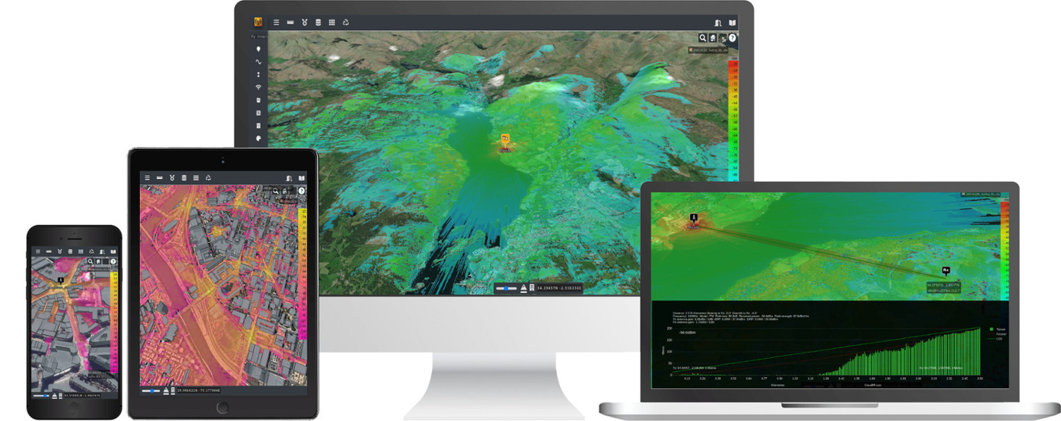
The 3D interface is the primary user interface for Cloud-RF. This interface is compatible with the desktops, tablets and mobile phones. 3D Interface supports Android, Linux, Mac/OSX and Windows. Furthermore, it can adjust to any device - the old iPhone, desktop computer and more!

To access the Cloud-RF 3D Interface, - Click on the Web Interface button on the Home Page. - The Performance Mode dialog box will appear.

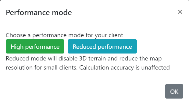
• Choose a Performance Mode as per your requirement.

  • You may select High Performance or Reduced Performance mode.

    If you choose the Reduced Performance mode, the 3D terrain will be disabled and the map resolution will be reduced. However, the calculation accuracy will remain the same as in High Performance mode.

3D Interface Elements

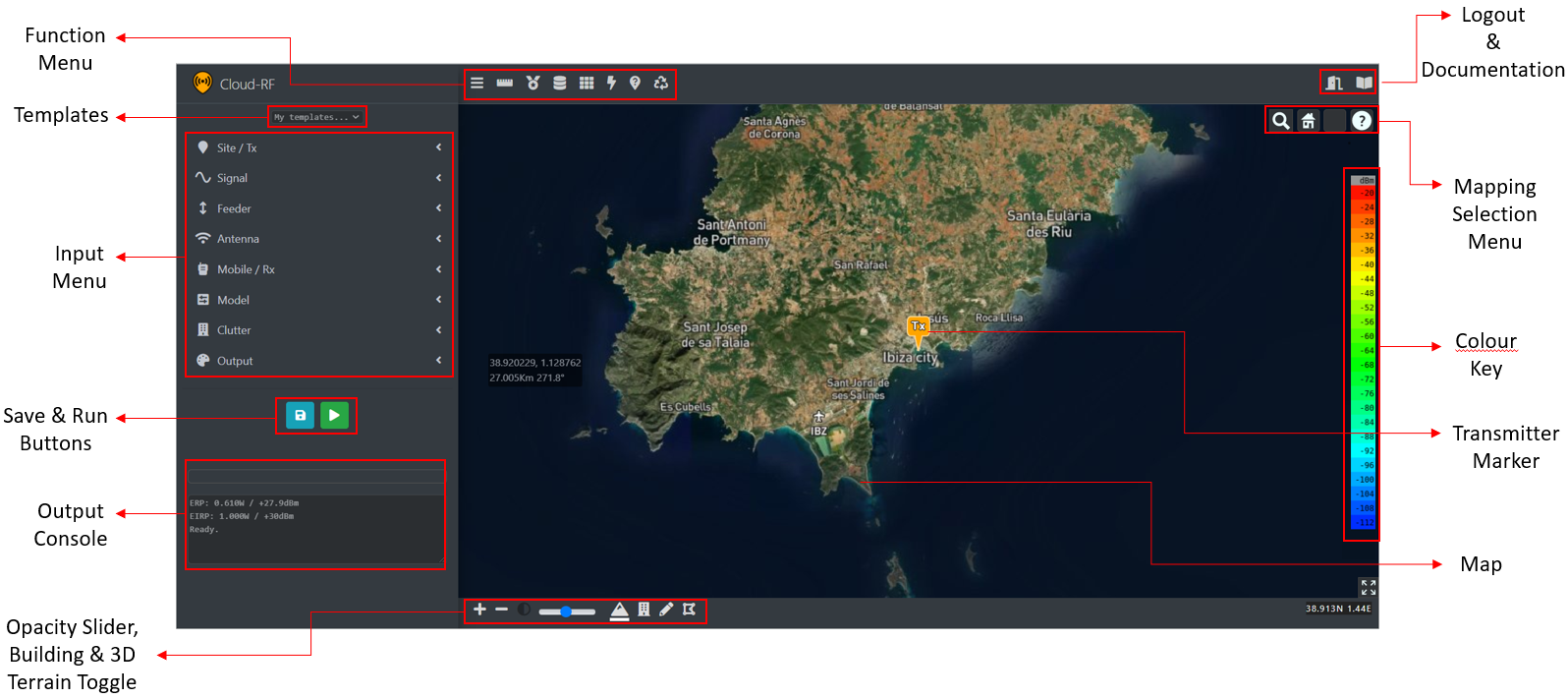
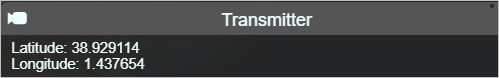
Transmitter Marker

The Transmitter Marker (Tx) indicates your Antenna Location.

To update your antenna location settings, - On the map, click on the desired location. - The transmitter marker will move to your clicked location. - The location settings under the input menu will be updated respectively.

• Click on the transmitter marker to view the location parameters of the Transmitter - Latitude and Longitude.
  

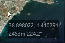
• When you have a layer, the information box next to the cursor will display the current co-ordinates, signal strength, distance and angle from the site.
  

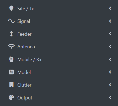
Input Menu

The Input Menu is an accordion style menu consisting of various collapsible sections with input fields. It allows you to focus on several settings which are further grouped into the various categories making it user-friendly.

The fields in the various input menu categories have a Help icon beside them. To know the details regarding a field, you can click on the Help icon of the respective field.

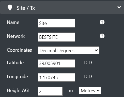
Site / Transmitter

The Site/Transmitter input menu consists of the settings related to the physical location of the antenna. These settings are relative to the ground and the Name & Parent of the site.

The Site/Tx settings will be of greater importance as your network grows and you need to perform analysis such as the best server analysis.

You can set location in the following two ways: - Manually - You can enter the Location fields (Latitude and Longitude) manually in the respective fields. > All the Inputs in the form of Decimal degrees, Degrees/Minutes/Seconds and NATO MGRS are acceptable. The system will make necessary conversions automatically.

OR - Clicking on the Map - You can click on the map and the location fields will be set accordingly.

Configure the following Site/Tx fields: - Name - Enter the desired unique name for your site. - Network - Enter the network name for logical grouping (as per the cities/area) of your site(s). - Coordinates - Select the desired coordinate format from the drop-down. - Latitude and Longitude - These location fields can be entered manually or set automatically by clicking on the map. - Height AGL - Enter the height (in metres or feet) above the surface model.

The Distance units applying to all heights and radiuses are set here. The default units of the system are Metre and Kilometre. Choosing Feet unit will set the distance calculations to Miles.

Signal

The Signal input menu consists of the settings related to the actual radiation.

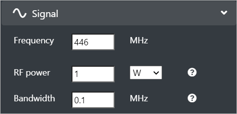
Configure the following Signal fields: - Frequency - Enter the system frequency (MHz) in the range: 20 to 100000 MHz. - RF Power - Enter the transmitter power (watts or dBm) before feeder loss and antenna gain. > ERP will be auto-calculated and displayed in the output console.

• Bandwidth - Enter the channel bandwidth (MHz).
  • Bandwidth will affect Channel Noise and Signal-to-Noise ratio.
  • Wideband channels will incur increased channel noise and reduced Signal/Noise Ratio. > The system will compensate for wide-band noise by making adjustments to the receiver sensitivity inline with Shannon’s theorem. Hence, the wideband signal would not appear to go as far as a narrow one – but the ERP/EIRP will be untouched.

Feeder

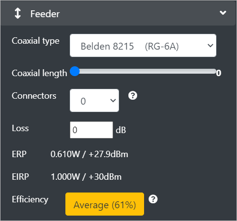
The Feeder input menu consists of the settings related to the cabling & connectors between a transmitter and a radio.

The theory - “Mounting an antenna higher always guarantees a better signal” does not always stand true. This theory only stands true when you are working at lower frequencies or have a very thick ‘low loss’ cable.

For UHF signals above 300MHz, feeder loss is a significant issue which must be budgeted carefully.

Configure the following Feeder fields:

• Coaxial Type - Select the Coaxial standard from the drop-down as per your requirement. The Coaxial Cable used will affect the feeder loss. > This can be safely ignored if the antenna screws directly onto the radio.

• Coaxial length - Set the slider to the desired Coaxial length of the cable. The cable length will significantly affect the feeder loss. Even a few metres of coaxial could reduce your system efficiency by 50%.

  This can be safely ignored if the antenna screws directly onto the radio.

• Connectors - Select the number of connectors from the drop-down as per your requirement. > This will affect the feeder loss.

• Loss - Enter the computed feeder loss in decibels. This must typically be in the range: 3 to 12dB. > If the feeder loss is more than 15dB, it indicates that your system is very inefficient.

• ERP and EIRP- The dynamically calculated Effective Radiated Power (ERP) and Effective Isotropic Radiated Power** (EIRP) will be displayed in the respective fields. > The ERP and EIRP values will change as you manipulate the powers and gains on the interface.

• Efficiency - This label will display the computed efficiency for your system based upon the RF input power and the computed ERP.

Antenna

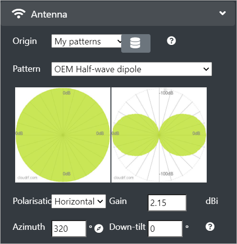
The Antenna input menu consists of the settings that lets you choose or build an antenna.

Configure the following Antenna fields:

• Origin - You can select My Patterns (system template) or Custom Pattern option from the drop-down. A custom pattern lets you build an antenna using beamwidth values in degrees.

  • If you select the Custom Pattern option,
    • You can configure the fields - Beamwidth (horizontal and vertical), Gain, Front-to-back ratio (use gain if unsure), Down-tilt relative to the horizon and Azimuth relative to true north.

  For further information, refer Custom Antenna Pattern Generation topic.

• Antenna Pattern database - Explore thousands of patterns in the database and select favourites to appear on your pattern select list. > For further information, refer Antenna archive - searching and favouriting a pattern topic.

• Polarisation - You can select Vertical or Horizontal option from the drop-down.

  The ITM model considers polarisation. Tx and Rx must match for optimal efficiency.

• Gain - Enter the antenna gain relative to an isotropic radiator. A dipole is 2.15 dBi > The peak gain is measured in decibel-isotropic (dBi) and will affects the ERP. For further information, see Feeder input menu.

• Azimuth - Enter the horizontal direction of the main lobe relative to grid north (in degree).
  • You can disable this in path profile mode so it always points along the path by clicking on the Compass icon.
  • To enable it, click on the Compass icon again.

• Down-Tilt- Enter the vertical direction of the main lobe relative to the horizon. > A positive value is towards the earth and a negative value is towards the sky.

• Custom: Horizontal Beamwidth - Enter the beamwidth in degrees between the half power (-3dB) points on the pattern in the horizontal plane.

• Custom: Vertical Beamwidth - Enter the beamwidth in degrees between the half power (-3dB) points on the pattern in the vertical plane.

• Polar Plots - The polar plots of the antenna pattern will update as you change the settings so you can see if it looks right.

• Custom: Front to back ratio - Enter the Ratio in decibels between the forward and rear gain values of a pattern. Use gain value if unsure.

  Ensure you set a positive gain and front-to-back ratio when building a custom pattern.

Custom Antenna Pattern Creation

You can create custom antenna pattern as per your requirement.

To do so,

• Click on Manage my Antennas icon.

  • The Antenna Database screen will appear in a separate tab.
    

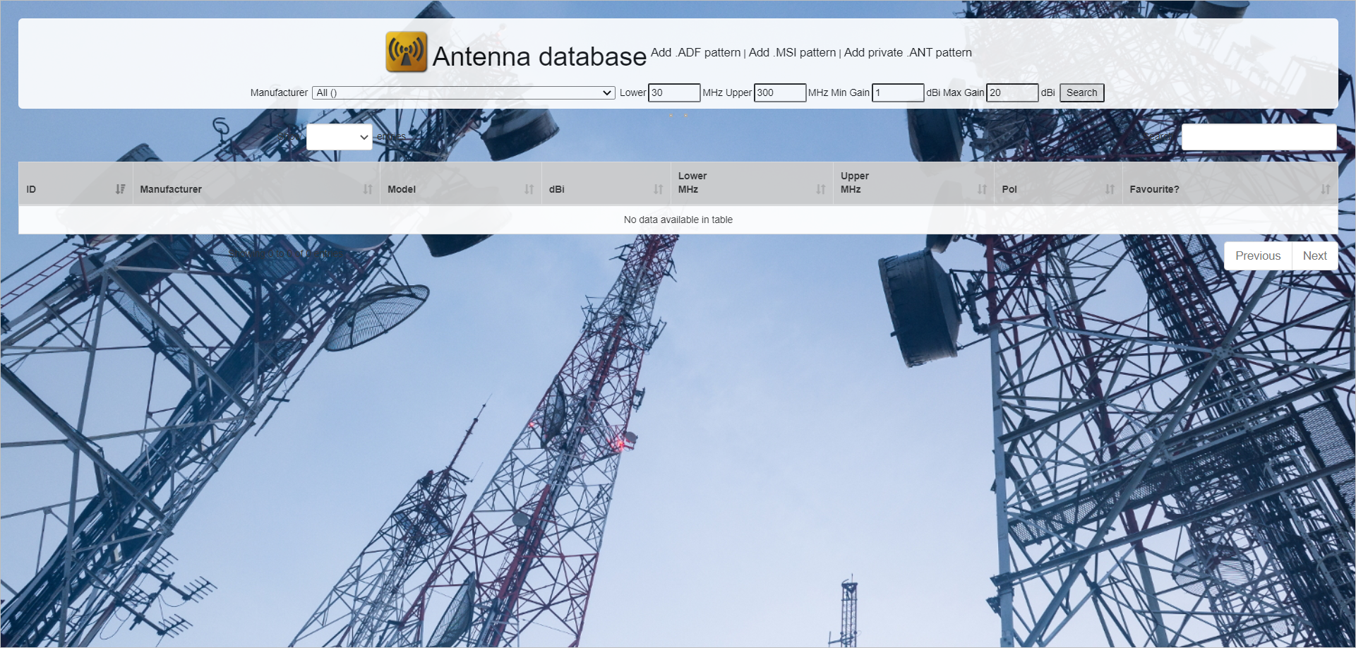
• You can either Search and Favouritize an Antenna Pattern or upload your desired antenna patterns to add them to your custom list and refresh the interface to have them populate in your list. > For Searching and Favouritizing, refer to the Searching and Favouriting an Antenna Pattern topic.

  • To add a desired antenna pattern,
    • Click on the respective link:
      • Add .ADF pattern
      • Add .MSI pattern
      • Add private .ANT pattern
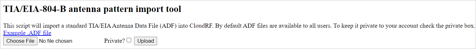
  • The respective Antenna Pattern Import Tool screen will be displayed.
    

• Click on Choose File button to browse and select the desired file to upload. > On the .ADF Pattern Import Tool screen , if you wish to keep the uploaded .ADF file private to your account, select the Private? checkbox.

• Click on the Upload button. #### Searching and Favouriting an Antenna Pattern

• To access the Antenna Database,
  • Click on the Manage my Antennas icon.
    • The Antenna Database screen will appear in a separate tab.
      
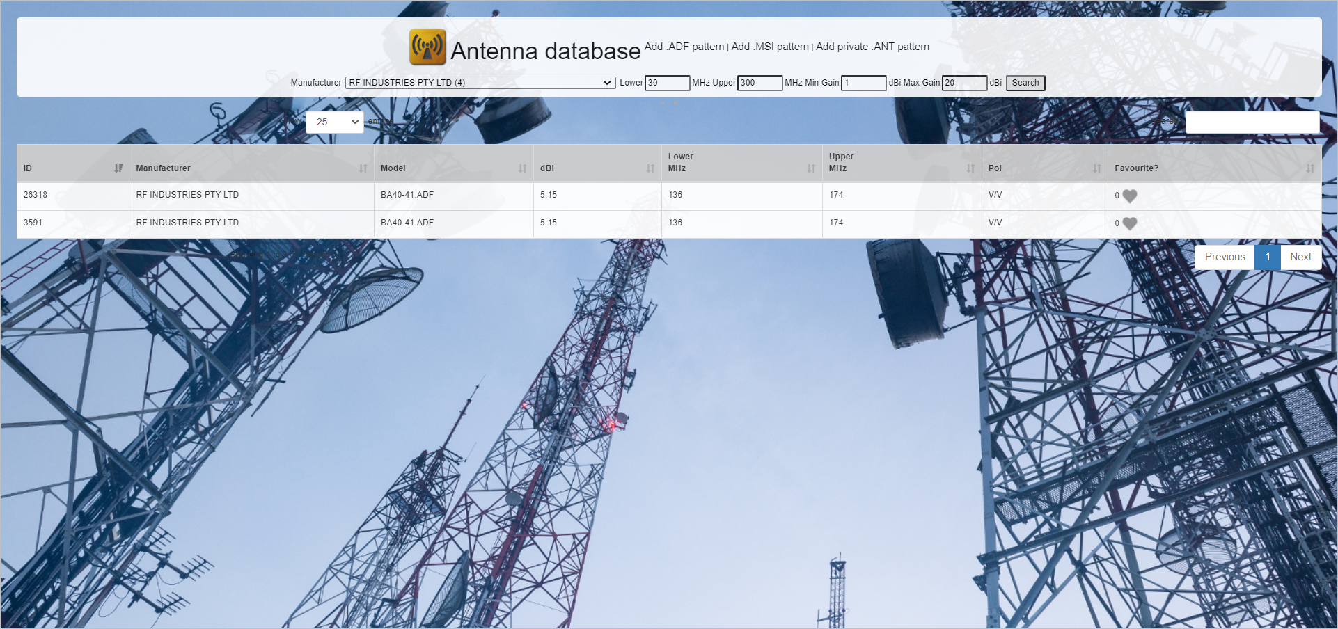
• To Search an Antenna Pattern,
  • Select the Manufacturer from the drop-down.
  • Configure the Lower, Upper (in MHz), Min Gain, Max Gain (in dBi) fields.
  • Click on the Search button.
  • The filtered entries will be displayed in a tabular form.
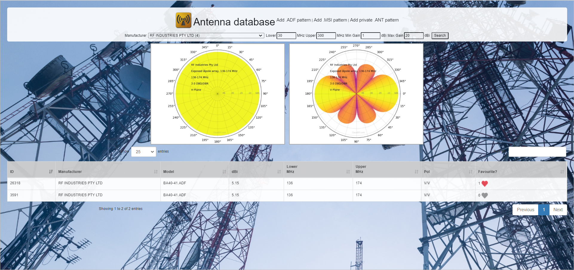
• For Favouriting an Antenna Pattern,
  • Click on the Favourite icon of the respective entry in the table.
  • The icon will turn red , indicating that the respective Antenna Pattern has been favouritised.
    • The polar plots of the favouritised antenna pattern in both Horizontal and Vertical planes will be displayed.
      

Mobile / Receiver

The Mobile/Receiver input menu consists of the settings related to the other end of the link. This could be a mobile outstation, a customer or a vehicle.

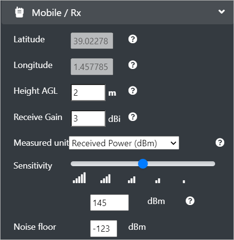
Configure the following Mobile/Rx fields:

• Latitude and Longitude - These location fields will be disabled by default.
  • To enable the fields, you can click on the Path Profile tool icon on the Function Menu.
  • The Latitude and Longitude fields will be enabled.
  • You can set the Receiver (customer) location by one of the following ways:
    • Click on the map.
    • The Latitude and Longitude field values will be set automatically. OR
    • Enter the values manually.
    • Click on the Run button.

• Height AGL - Enter the height above ground level (surface model) in metres or feet. > The Height units (metres/feet) can be set under Site/Tx Input Menu in the Height field.

  For example: If the surface model is LIDAR that includes a 30m building and your mobile station is 4m on the roof then Height AGL will be 4m. If LIDAR is not present, then Height AGL will be 34m.

  For a handheld radio, you can use the Height AGL values as 1m or 2m.

• Receive Gain - Enter the receive gain in dBi. This is the combined receiver and antenna gain. The receiver gain considers the antenna, receiver noise and (receive) feeder loss.

  For example: If the receiver has a 3dBi antenna and a 3dBi receiver noise figure, the Receive gain would be 0 dBi.

  For a Mobile Phone, you can use the Receive Gain value of 1dBi. The actual performance varies by band, so a phone may have 2dBi gain for GSM900 but 1dBi for UMTS-2100.

• Measured units - Select the output units option from the drop-down as per your requirement. The measured units can either be in dB, dBm or dBuV/m.

  While the Received power (dBm) is the most popular unit for coverage maps, the Field Strength (dBuV) is often used for compliance purposes.

  The units must correspond with the selected colour key if performing area coverage plots.

• Sensitivity - Set the sensitivity slider to define the sensitivity of the mobile station in units corresponding to the measured units.

  SET WITH CARE.

  Use -90dBm if unsure.

  A mobile phone’s sensitivity is between -100dBm and -115dBm. Setting the sensitivity too low (eg. -120dBm) would result in an unrealistic prediction unless your system is designed to function that low.

  IoT protocols like LoRa LPWAN can theoretically operate down to -140dBm but this is under ideal conditions. In the real, noisy world, most digital communications bottom out at between -100 and -115dBm. Adding a 10dB error margin gives a recommended range of -90 to -105dBm for sensitivity.

• Noise floor (SNR units only) - Enter the thermal noise floor value in dBm. It is used in conjunction with the required SNR to establish the sensitivity.

  A QPSK threshold is 4dB whilst the noise floor can vary between -100 and -130dBm. Use -120dBm if unsure.

Model

The Model input menu consists of the settings related to the Propagation Model.

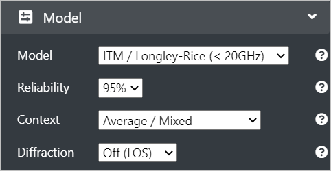
Configure the following Model fields:

• Model - Select the Propagation model from the drop-down as per your requirement. > While the ITM model is recommended for planning over complex terrain, the Free space model is ideal for a microwave link.

• Reliability - This field is applicable only to ITM model. You can select the reliability percentage as per your requirement. > 99% indicates a conservative ‘high confidence’ prediction. > 90% indicates an optimistic prediction. > 95% is the default set value.

• Context - Select the context of the model from the drop-down as per your requirement. Many models have environmental variables which provide different outputs.

  Tip: For a conservative output, select Conservative/Urban as the option. Else, keep the default Average/Mixed option.

• Diffraction - You may select the diffraction option as knife-edge to post-compute diffraction after an obstacle. Default option is Off(LOS).

  The radio shadow size will vary by frequency and obstacle distance/height.

  Not required for ITM.

Clutter

The Clutter input menu consists of the settings related to the system clutter.

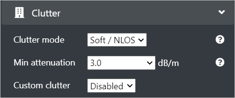
Configure the following Clutter fields:

• Clutter mode - Select the Clutter mode option from the drop-down as per your requirement.

  • If you select Hard/LOS , only the line of sight coverage will be displayed.
  • If you select Soft / NLOS, then the coverage through an obstruction will be displayed.

  The density is defined within the system clutter or can be overridden with an average attenuation value.

• Min attenuation - Select the Clutter attenuation option from the drop-down as per your requirement. > This field is enabled only if you have selected Soft/NLOS as the Clutter mode.

  The Clutter Attenuation is a mean value (in dB/m) calculated by penetrating a signal of 1GHz from a building with exterior & interior walls along with a lot of free space in between.

  For example: A 10m house with 2x 7dB brick walls and 2x 3dB partition walls would have an average of 2.0dB/m.

  • For planning purposes, you can select:
    • 5.0dB/m for concrete buildings.
    • 1.0dB/m for timber houses. > Trees vary by season and type but can be in range: 0.01dB/m to 0.3dB/m.

Output

The Output input menu consists of the settings related to the system output.

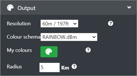
Configure the following Output fields:

• Resolution - Select the desired resolution from the drop-down as per your requirement. Make sure that the resolution when combined with the radius to compute a mega-pixel value, is within your plan limit.

  2m is not recommended unless you know that the city or area supports this data via LIDAR. TIP: 16m presents a much better compromise for accuracy in most countries due to proximity to the underlying surface model.

• Colour Schema - Select the colour schema by clicking on the Manage my colours icon.

  • The My Colours screen will be displayed.

    For further information, refer ** Colour pattern generation using colour tool** topic.

• Radius - Enter the desired radius(in Km). This value is used with resolution to compute mega-pixels which are displayed in the corner console. For example: 5km radius calculation at 2m resolution would result in 25MP image. Similarly, 5km@10m = 1 MP.

  TIP: Do not request a non-practical calculation. For example, you cannot request a 20km radius calculation at 2m resolution as this would create a 400 mega pixel image which is not practical.

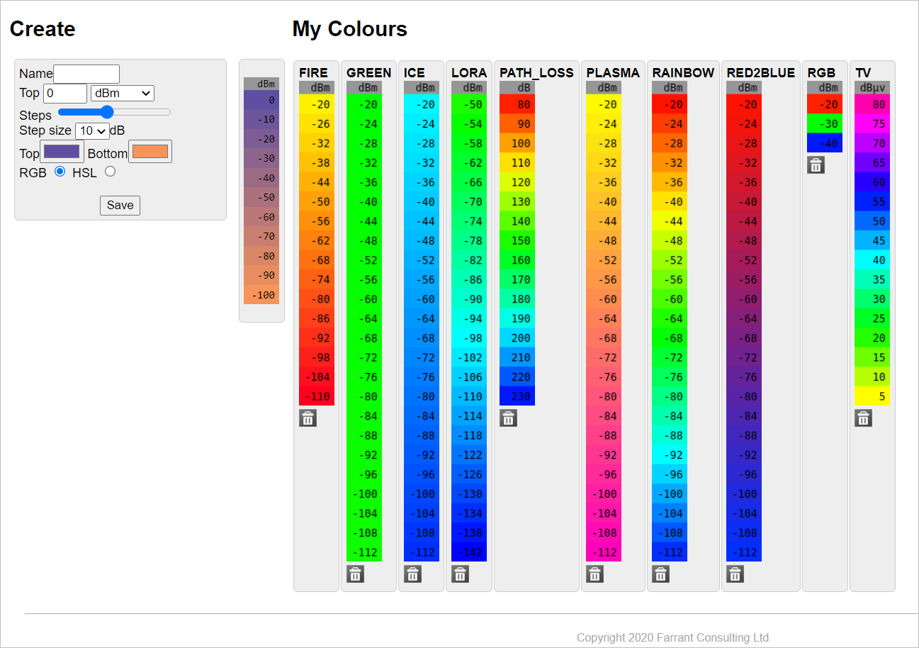
Colour pattern generation using colour tool

You can create custom colour pattern as per your requirement, edit the colour keys, set levels, change colours and define limits.

To create custom colour pattern, - Select the colour schema by clicking on the Manage my colours icon. - The My Colours screen will appear in a separate tab.

• You may create a customized colour pattern.

To do so, - In the Name field, enter the desired name for the new colour schema. > To edit an existing pattern, enter the colour pattern name here. You may edit the fields as per your requirement.

• In the Top field, enter the top-most value of the colour pattern.
  • Select the desired colour pattern unit (dB, dBm or dBµV/m) from the drop-down.
• In the Steps slider, set the number of steps you wish to be displayed in the colour pattern.
• In the Step size field, select the size of the step as per your requirement.
• In Top and Bottom fields, select the colour shade that you wish to get displayed at the top and bottom of the colour pattern.
  • Select the colour codes (RGB or HSL) radio buttons that you wish to use in your customized colour pattern.
• Click on Save button.
• The following dialog box will be displayed.
  

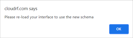
• Click on the OK button.

  To view the new created colour pattern or the changes made in the existing schema, you must reload the interface.

Save and Run Buttons

After configuring the Input Menu, you can Save and Run the configuration by clicking on the respective button.

These buttons are displayed below the Input Menu.

Save

Save button lets you create a template with all your configured settings that you can reuse later whenever required. > For further information, refer Templates topic.

Run

Run button will execute a coverage calculation using your configured settings. - The execution may take several seconds depending on the resolution and the radius. The Progress Bar will be displayed in this case. - In case there are errors in the configuration, the respective error dialog box will appear. - Make the necessary corrections and re-run the updated configuration.

• After successful execution, the Site name (Network name) field will be displayed in the Output Console. > For further information, refer the Output Console topic.

Templates

Templates allows you to quickly apply settings from a saved configuration.

Saving a Template

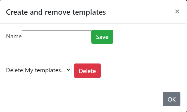
To save a Template, - Configure the Input Menu as per your requirement. - Click on the Save button. - The Create and Remove Templates dialog box will appear.

Creating a Template

To create a Template, - After configuration in the Input Menu, click on the Save button. - In the Create and Remove Templates dialog box, - In the Name field, enter the desired Template name. > You can give a user-friendly name, for example: “Radio X”.

- Click on **Save** button.

• The created Template will be displayed under My Templates drop-down. > This is useful in a shared account where an Engineer might prepare the template(s) and a sales person might use them to qualify customers.

Deleting a Template

To delete a Template, - Click on the Save button. - In the Create and Remove Templates dialog box, - In the Delete field, select the Template Name that you wish to delete. - Click on Delete button. - The deleted Template will be removed from the My Templates drop-down.

Output Console

The output console provides the useful feedback related to the settings, errors, API inputs and API outputs as you use the Cloud-RF tool.

• The Effective Radiated Power (ERP) and the computed resolution (in mega-pixels) will be printed in this console as you adjust the settings so that you can keep an eye on the same.

• As an area calculation processes, you will see periodic updates in the console from the SLEIPNIR propagation engine.

• When you submit a calculation for processing, all the API parameters will be displayed here. If you are a developer, you can directly copy paste this to use it in your code.

• To do so,

  • Click on the Run button for execution, the Site name (Network name) field will be displayed in the Output Console.
    

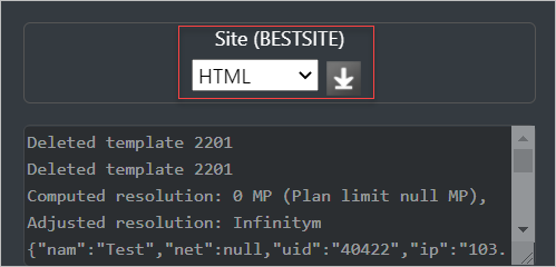
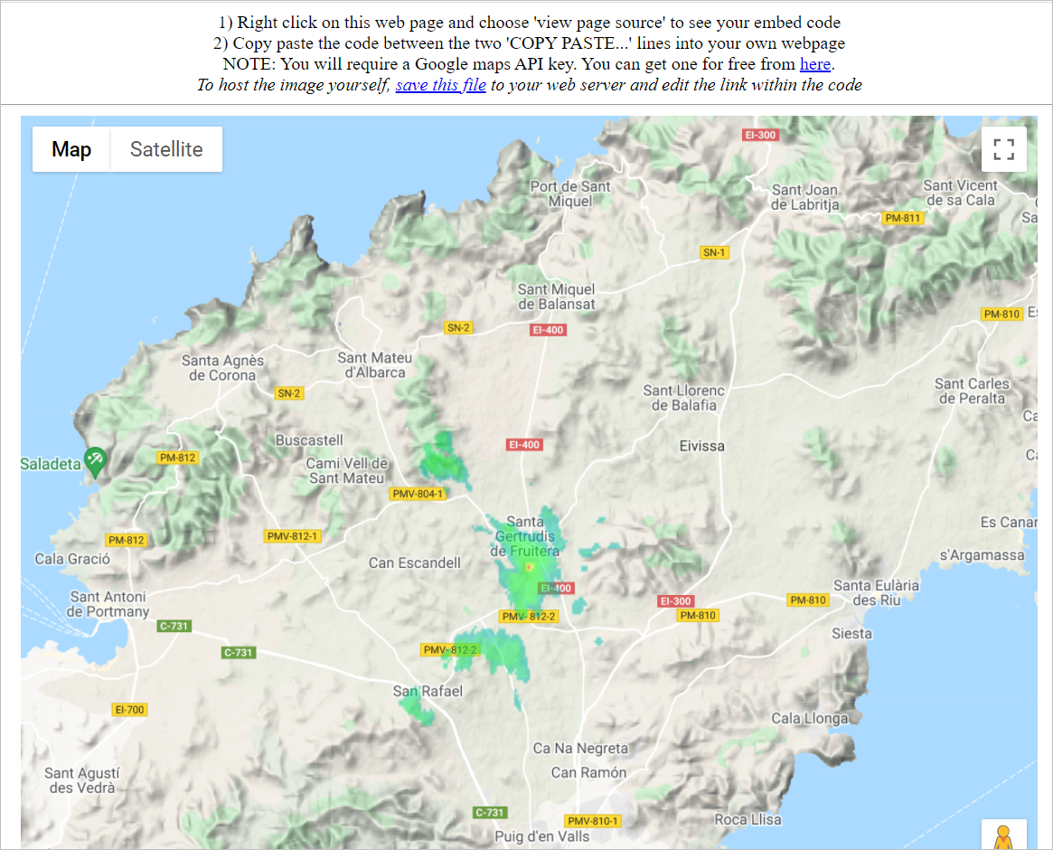
  • Select the file format in which you wish to download the configuration settings file. - Click on Download icon. - If you download this in HTML Format, the following screen will appear in a separate tab.
    

Function Menu

The Function Menu is a set of various key functions located on the top of the interface. Each function has a designated clickable button that allows you to locate them easily on the interface, thus making the tool easy-to-use and user-friendly.

Function Menu Elements

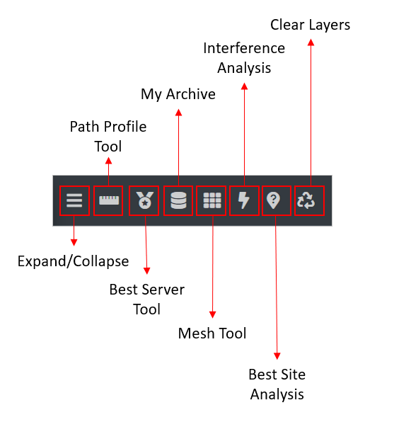
Expand/Collapse

The Expand/Collapse button lets you expand or collapse the Side Menu consisting of Templates, Input Menu and Output Console.

To Collapse the side menu, - Click on the Expand/Collapse button. - The Side Menu will collapse. > When you mouse-over upon the Side Menu, the expanded view of the menu will appear.

To Expand the side menu, - Click on the Expand/Collapse button. - The Side Menu will expand.

Path Profile Tool

The Path Profile Analysis tool lets you inspect the terrain profile between two positions - Transmitter and Receiver.

Point-to-Point Path Profile Analysis (Tx to Rx)

For Point-to-point path profile analysis (Tx to Rx), you can set the Transmitter and Receiver location either by Visual Map Placement or Precise Location Entry method.

1. Visual Map Placement You can click on the Map to site your Transmitter and Receiver location visually. - Site your Transmitter location on the map. - Click on the Path Profile Tool button on the Function Menu. - Click on the map to site your Receiver location.

2. Precise Location Entry To use GPS co-ordinates, you can configure the Transmitter and Receiver location manually. - Configure your Transmitter location (Latitude and Longitude) in the Site/Tx Input Menu. - Click on the Path Profile Tool button on the Function Menu. - Configure your Receiver location in the Mobile/Rx Input Menu. - Click on Run button.

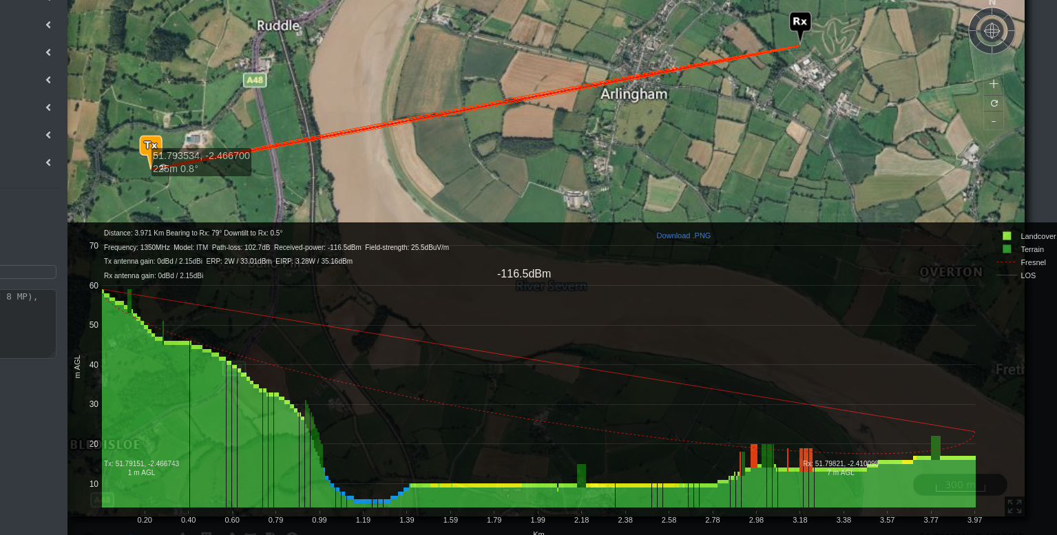
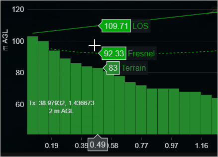
The Black Result Box After setting your Transmitter and Receiver location, the Black Result Box will appear.

• The Path Profile in the form of a graph consisting of the path profile components - Terrain, Fresnel and LOS will be displayed.
  

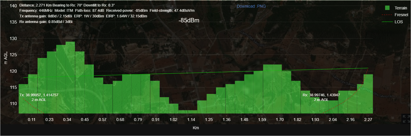
• The Transmitter and Receiver related information (Distance, Frequency, Model, Path Loss, Received Power, Field Strength, Tx Antenna Gain, ERP, EIRP, Rx Antenna Gain) will also be displayed along with the graph.
• You can click on the Download.PNG link to download the Path Profile graph image.

• Various Function Icons will be available as you mouse-over on the Result Box.
  

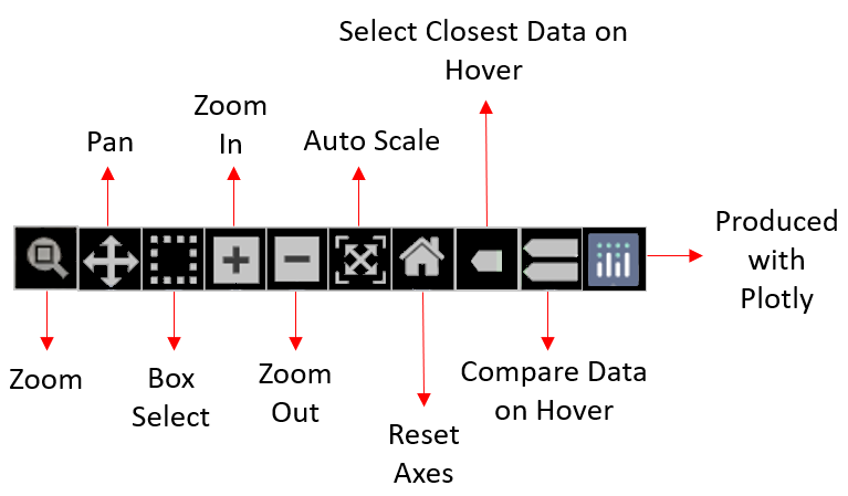
  • Zoom - lets you zoom the desired section of the Path Profile Graph. - Click on the desired section’s starting point and without releasing the mouse, select the section.
    • Pan - lets you pan view the graph interactively.
      • On selecting the Pan function icon, the pan mode for axes gets turned on in both x and y directions.
      • Click on the graph and without releasing your mouse, move in the direction you wish to pan view the Path Profile.
    • Box Select - lets you select a particular section of the graph that you wish to view.
      • The selected box section will be highlighted from the rest of the path profile graph for clear view.
    • Zoom In - lets you zoom in the Path Profile Graph.
    • Zoom Out - lets you zoom out the Path Profile Graph.
    • Auto Scale - lets you auto scale the axes of the graph.
    • Reset Axes - resets the axes as per the original graph.
    • Show Closest Data on Hover - shows you the closest data from the point on the graph where you hover.
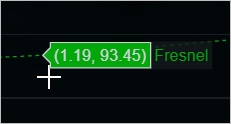
      • The closest path coordinate will be displayed as below:
        
    • Compare Data on Hover - shows you the comparison of the data from the point on the graph where you hover.
      • The graph comparison will be displayed as below:
        
    • Produced with Plotly - redirects you to the Plotly website.

To change the resolution, - Click on Output Input Menu. - In the Resolution field, select the resolution that you wish to set from the drop-down.

To change the building / clutter attenuation, - Click on Clutter Input Menu. - In the Clutter Mode field, select Soft/NLOS as the option from the drop-down. - In the Min attenuation field, select the Clutter attenuation that you wish to set from the drop-down.

Point-to-Multipoint Path Profile Analysis (Many Tx, one Rx)

Need more clarity regarding Point-to-Multipoint / Area (Big green button).

Best Server Tool

The Best Server Tool is useful for checking the coverage on an established network.

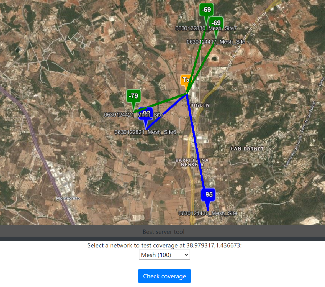
To use the Best Server Tool, - Click on the Best Server Tool button on the Function Menu. - The Best Server Tool dialog box will appear. - Site your Transmitter location on the map. - Select a network to test coverage at the set transmitter location from the drop-down. - Click on Check Coverage button. - The Network Coverage as per your transmitter location will be reflected on the map. - You can change your transmitter location on the map to check the best server location and the network coverage.

My Archive

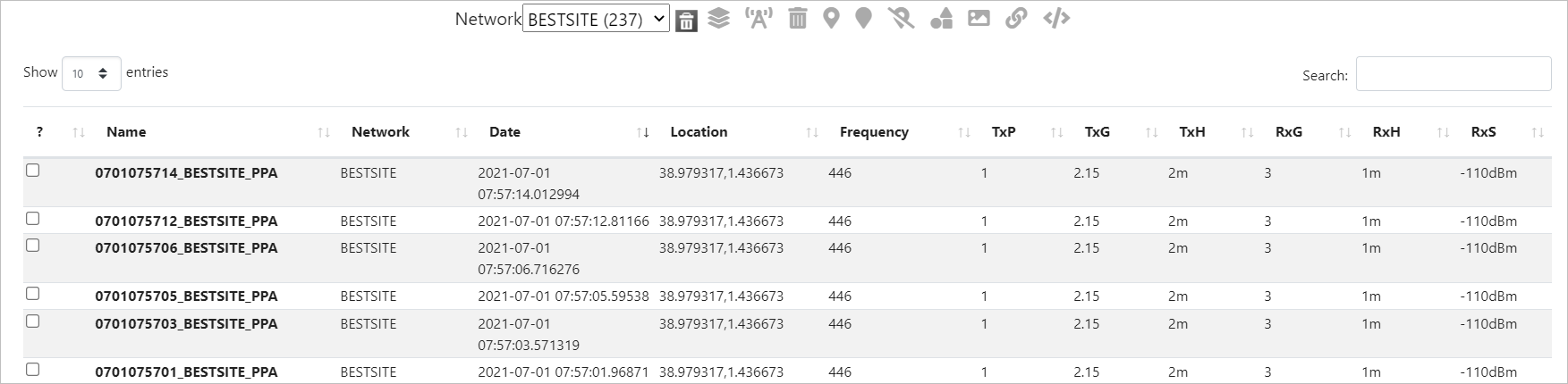
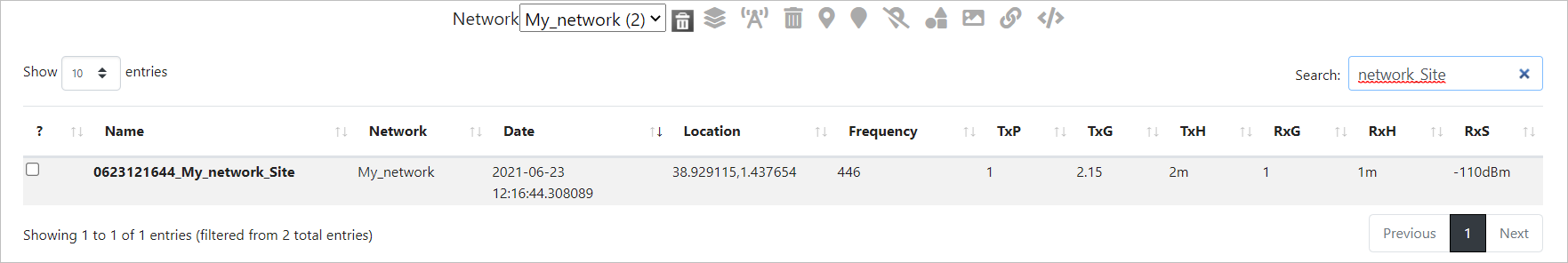
My Archive lets you view the list of your saved networks and their details.

• Click on My Archive button on the Function Menu.
• The My Archive dialog box will appear.
  

Searching and Filtering (Network Selection)

You can select and filter the Network(s) as per your requirement.

To do so, - Select the desired Network from the drop-down. - The respective Network entries in a tabular format will be displayed. - You may search the required network using the Search box. - The filtered entries will be displayed.

Sorting

You can sort the Network entries in ascending or descending order as per your requirement.

To do so, - Click on the Sort icon of the respective column. - The sorted entries will be displayed in the table. > indicates Sorting in the Ascending Order. indicates Sorting in the Descending Order.

• Various Function Icons are also available.
  

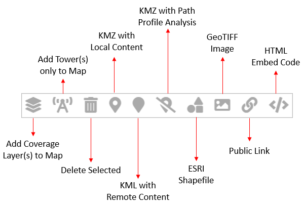
  • Add Coverage Layer(s) to Map - lets you add the selected network(s)’ coverage layer(s) to the map.
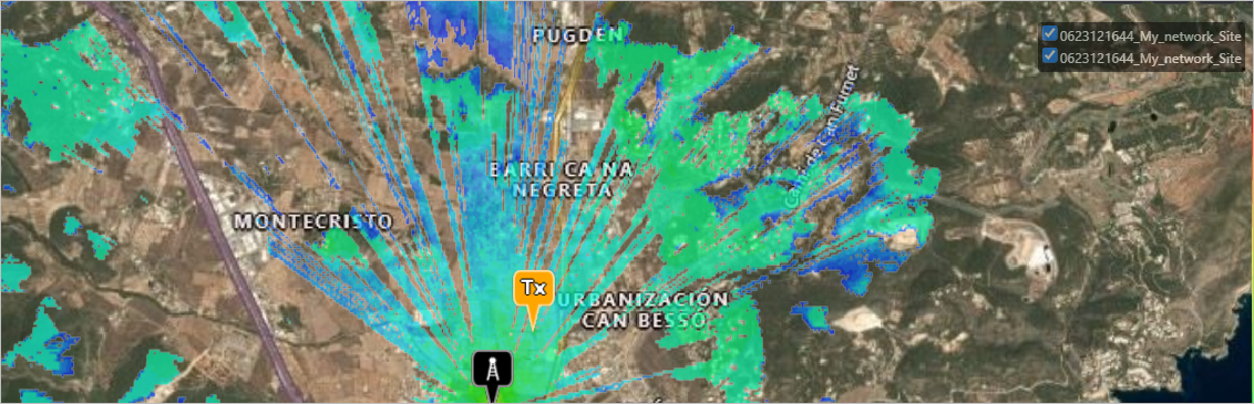    - You can manage (select/deselect) the network site locations by clicking on the respective checkbox.

  • Add Tower(s) only to Map - lets you add the tower(s) to the map in the selected network(s).
    • Delete Selected - lets you delete the selected Network(s).
      • When you click on the Delete Selected button, the following warning dialog box will appear.
        
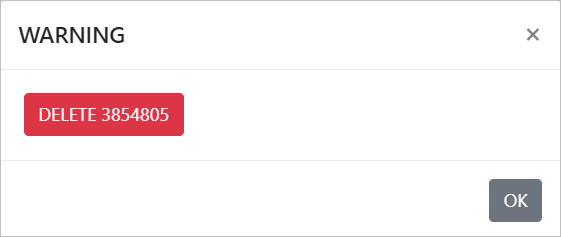
        • Click on OK button to confirm.
  • KMZ with Local Content - lets you download the KMZ file with the local content.
    • KML with Remote Content - lets you download the KML file with the remote content.
    • KMZ with Path Profile Analysis - lets you download the KMZ file with Path Profile Analysis.
    • ESRI Shapefile - lets you download the Coverage zip file consisting of the DBH, PRJ, SHP, SHX files of the selected network(s).
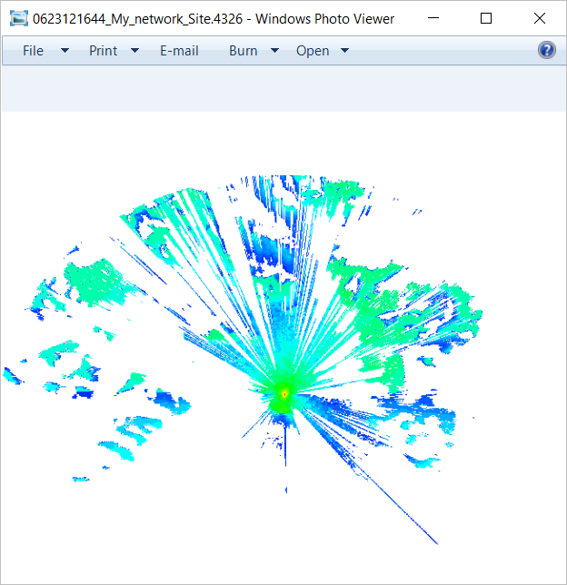
    • GeoTIFF Image - lets you download the GeoTIFF image of the selected network(s).
      

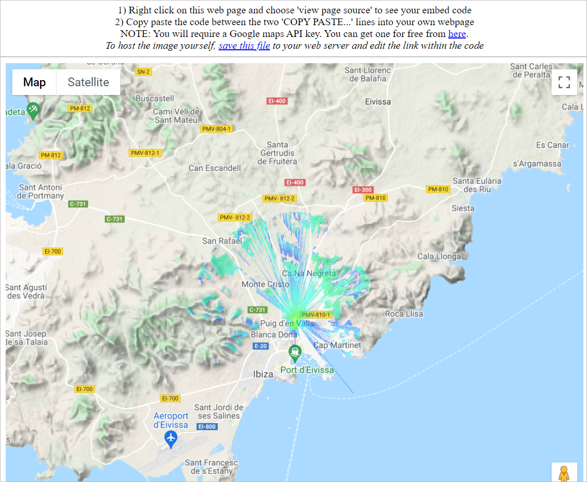
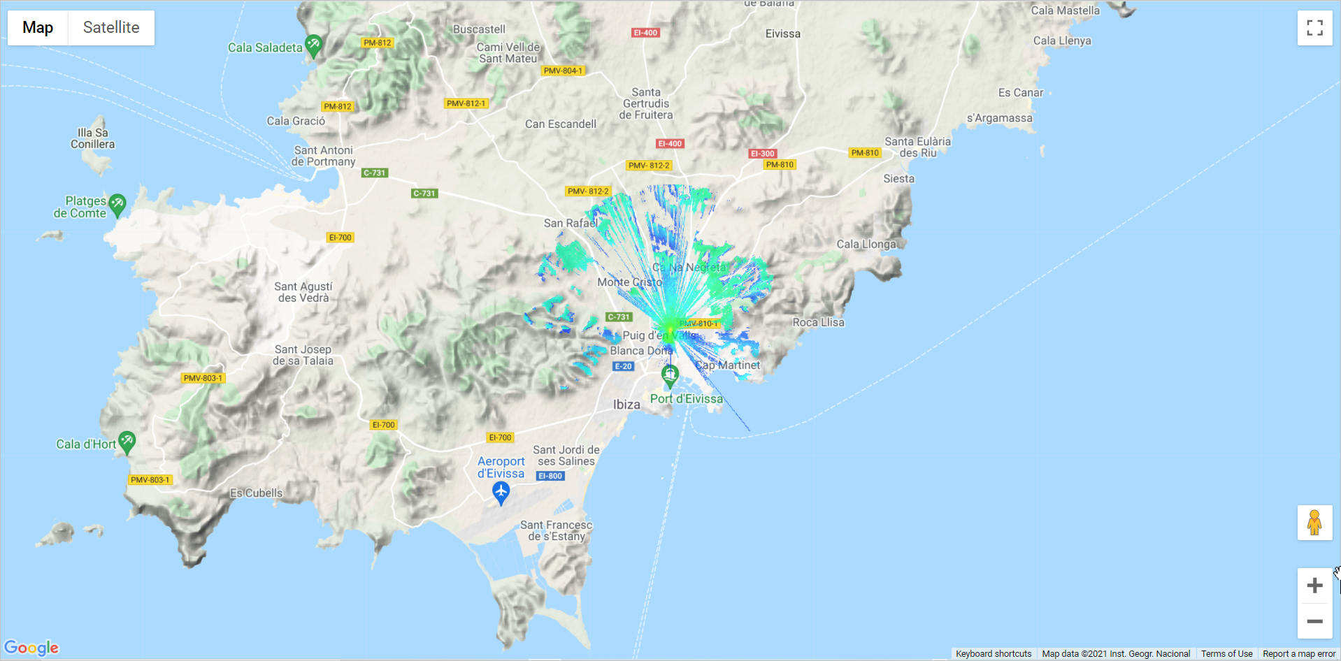
  • Public Link - lets you view the selected Network(s) in the Google Map.
    

  • HTML Embed Code - opens the following screen in a separate tab. All the API parameters of the selected network(s) will be displayed here. If you are a developer, you can directly copy paste this to use it in your code.